DOCUMENTOS DE ECONOMIA Y FINANZAS INTERNACIONALES

Determinants of regional integration agreements in a discrete choice

framework: Re-Examining the evidence

Laura Márquez-Ramos Inmaculada Martínez-Zarzoso

Celestino Suárez-Burguet

December 2005

DEFI 05/10

Asociación Española de Economía y Finanzas Internacionales

http://www.fedea.es

ISSN 1696-6376 Las opiniones contenidas en los Documentos de la Serie DEFI, reflejan exclusivamente las de los autores y no necesariamente las de FEDEA.

The opinions in the DEFI Series are the responsibility of the authors an therefore, do not necessarily coincide with those of the FEDEA.

DETERMINANTS OF REGIONAL INTEGRATION

AGREEMENTS IN A DISCRETE CHOICE

FRAMEWORK: RE-EXAMINING THE EVIDENCE

LAURA MÁRQUEZ-RAMOS*

lmarquez @eco.uji.es

INMACULADA MARTÍNEZ-ZARZOSO*

martinei@eco.uji.es

CELESTINO SUÁREZ-BURGUET*

celes@eco.uji.es

Departamento de Economía and Instituto de Economía Internacional

Universitat Jaume I

Campus del Riu Sec

12071 Castellón (Spain)

* We would like to thank Jeffrey Bergstrand for his helpful comments, and also participants in the European Trade Study Group conference held in Dublin and in the Atlantic Economic Conference held in New York. The authors acknowledge the support and collaboration of Proyectos BEC 2002-02083, SEJ 2005-01163, Bancaja-Castellón P-1B92002-11 and Grupos 03-151 (INTECO). Martínez-Zarzoso is grateful to the members of the Ibero American Institute for Economic Research in Goettingen for their hospitality.

2

Determinants of regional integration agreements in a

discrete choice framework: re-examining the evidence

Abstract

This paper provides new empirical evidence on the determinants of regional integration agreements

(RIAs) in a discrete choice modelling framework. The research has two main aims: first, to empirically

analyse the determinants of different levels of integration, re-examining the evidence presented by Baier

and Bergstrand (2004) in the JIE 64 (1); and second, to analyse the importance of additional factors, in

particular socio-political factors. The results show that geographical factors alone are the most important

explanatory factors for the probability of regional integration agreement formation or enhancement, thus

supporting the theories on “natural” trading partners. The socio-political factors considered, democracy

dummy, the level of economic freedom and the common language dummy are all statistically significant,

although their relative importance in explaining RIA formation is low.

Keywords: Regional integration agreements, discrete choice models, trade flows, natural partners

JEL classification: F11, F12, F15

1. Introduction

A major concern in the traditional literature on the formation of free trade areas (FTAs)

has been whether these areas generate welfare gains for the individual countries that

engage in these processes. Since the 1950s (Viner, 1950) many authors have contributed

to this debate, and especially in the 1990s, studies based on the gravity model

proliferated (Frankel, Stein and Wei –FSW-, 1995, 1996, 1998). However, none of this

research has attempted to evaluate the determinants of FTA formation.

Only recently have Baier and Bergstrand (2004) developed the first theoretical and

empirical analysis of the economic determinants of FTA formation. They provide an

economic benchmark for future political economy models to explain the determinants of

FTAs. They find evidence showing that pairs of countries will be more likely to form

FTAs if they share the following characteristics: a) they are geographically close to each

3

other, b) they are remote from the rest of the world, c) they are large and of similar

economic size, d) the difference of capital-labour between them is large and e) the

difference of their capital-labour ratios is small compared to the rest of the world. Baier

and Bergstrand (BB) only consider whether or not each pair of countries is involved in

an FTA. Therefore the variable they attempt to explain is binary and takes the values

zero and one. Baier and Bergstrand (2005) show the importance of treating FTAs as

endogenous when the determinants of trade flows are analysed. They show that when

the endogeneity of the FTA variables is taken into account in gravity models, their

effect on trade flows is quintupled.

We extend BB’s work in two ways: firstly, we investigate the determinants of regional

integration agreements (RIAs) rather than FTAs by considering five different levels of

integration between pairs of countries: Preferential trade agreement (PTA), free trade

agreement (FTA), customs union (CU), single market (SM) and monetary union (MU).

Secondly, we address the importance of additional economic, geographical and socio-

political variables as determinants of RIAs.

We begin by replicating the BB empirical work to verify the robustness of their results

with an alternative data set. We then estimate an ordered logit model (instead of a

binary probit) with the same explanatory variables considered by BB to benchmark our

extension to their original work. Finally, the ordered logit is estimated with additional

economic, geographical and socio-political variables. The economic variables we

consider are economic size, income differences, factor endowment differences and trade

barriers. Adjacency and landlocked status are added to BB’s list of geographical

variables. The socio-political variables are a shared language, political regime and level

of economic freedom.

4

We find that: (i) BB’s results are fairly robust, although with our data base the K -L

difference variable shows a reversal of the coefficient signs; (ii) the additional

characteristics considered have a significant impact on the probability of an RIA being

formed; (iii) as BB stated, socio-political factors are less important than economic and

geographical factors.

To our knowledge, Wu (2004) is the only author to have considered different levels of

integration ranked across countries. However, her paper focuses on the role that political

and economic uncertainty plays in explaining RIA formation and her results are not

directly comparable to Baier and Bergstrand since she includes different explanatory

variables in her model. Wu shows that countries’ per capita income, democracy and

geographical characteristics appear to be the best indicators of the probability of

participation in a certain level of RIA in the period 1987-1998. Surprisingly, Wu (2004)

does not consider the distance variable as a determinant of RIA formation. This

omission may influence the results obtained for other variables, since the model is not

well specified.

The remainder of the paper is structured as follows. Section 2 presents the theoretical

framework and the econometric model. Section 3 describes the data, the variables and

the hypothesis to be tested. Section 4 discusses the estimation results and Section 5

concludes.

2. Theoretical framework and econometric model

2.1 The theory

We take as our theoretical framework the Baier and Bergstrand (2004) model, which is

a generalisation of the Krugman-FSW model. The model allows for asymmetries

between countries and sectors and considers positive intra- and inter-continental

transport costs.

5

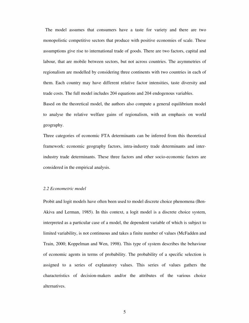
The model assumes that consumers have a taste for variety and there are two

monopolistic competitive sectors that produce with positive economies of scale. These

assumptions give rise to international trade of goods. There are two factors, capital and

labour, that are mobile between sectors, but not across countries. The asymmetries of

regionalism are modelled by considering three continents with two countries in each of

them. Each country may have different relative factor intensities, taste diversity and

trade costs. The full model includes 204 equations and 204 endogenous variables.

Based on the theoretical model, the authors also compute a general equilibrium model

to analyse the relative welfare gains of regionalism, with an emphasis on world

geography.

Three categories of economic FTA determinants can be inferred from this theoretical

framework: economic geography factors, intra-industry trade determinants and inter-

industry trade determinants. These three factors and other socio-economic factors are

considered in the empirical analysis.

2.2 Econometric model

Probit and logit models have often been used to model discrete choice phenomena (Ben-

Akiva and Lerman, 1985). In this context, a logit model is a discrete choice system,

interpreted as a particular case of a model, the dependent variable of which is subject to

limited variability, is not continuous and takes a finite number of values (McFadden and

Train, 2000; Koppelman and Wen, 1998). This type of system describes the behaviour

of economic agents in terms of probability. The probability of a specific selection is

assigned to a series of explanatory values. This series of values gathers the

characteristics of decision-makers and/or the attributes of the various choice

alternatives.

6

Multinomial logit or probit models are used when there are more than two alternatives.

However, they fail to account for the ordinal nature of the dependent variable used in

this research. We aim to model the choice of sequential binary decisions, the first one

consisting of a pair of countries that either sign a preferential trade agreement (PTA) or

do not. Once a country has a bilateral agreement, the next decision will be whether to

take a further step and go to a higher level of integration. Therefore, the model objective

is to take a series of binary decisions, each one consisting of the decision of whether to

accept the current value or “take one more”. In this context, Amemiya (1975) describes

a model that applies to ordered discrete alternatives, such as the number of cars owned

by a household. This is based on the assumption of local (as opposed to global) utility

maximisation. The decision maker stops when the first local optimum is reached.

Economic agents must choose between two sequential options, and their selection

depends on their characteristics and their environment. In accordance with the

characteristics of our dependent variable, an ordered logit model was specified in our

study.

The model is built around a latent regression in the same way as the binomial probit

model. An observed ordinal variable, Y, is a function of a unobserved latent variable,

Y*, which represents the difference in utility levels from an action. The continuous

latent variable Y* has a number of threshold points, and the value of the observed

variable Y depends on whether or not a particular threshold is crossed. In the present

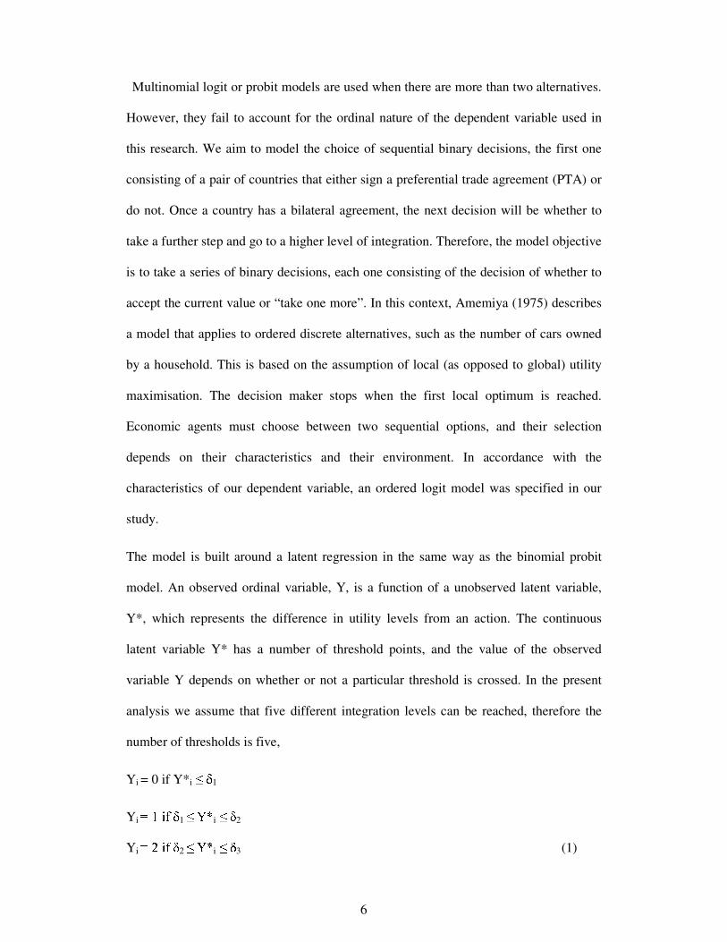
analysis we assume that five different integration levels can be reached, therefore the

number of thresholds is five,

Yi = 0 if Y*i � �

1

Yi ������� 1 � � � i � � 2

Yi �������� 2 � � � i � � 3 (1)

7

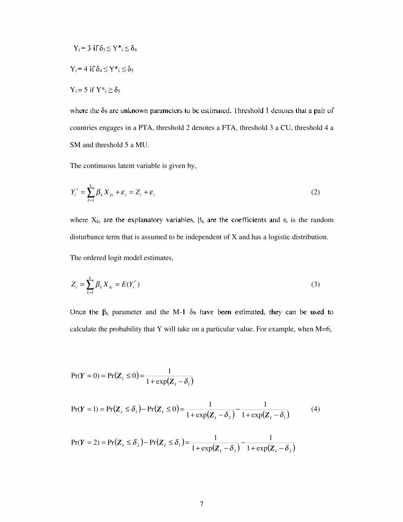
Yi ������� 3 ! "$# i ! 4

Yi %�&�'�() 4 * + , i * ) 5

Yi = 5 if Y*i - . 5

/10325462879032;: <>=5?A@CBEDEFGD3HJIKD�LM=N?6=NOP@NQR@N?S<TQUHWV3@;@X<AQZY[O$=5QU@]\_^a`cbE?6@X<SbMHGd�\�e8\f@NDMHgQU@a<cQ9b3=NQ_=hLG=gY[?iHEjcountries engages in a PTA, threshold 2 denotes a FTA, threshold 3 a CU, threshold 4 a

SM and threshold 5 a MU.

The continuous latent variable is given by,

∑=

+=+=k

kiiikiki ZXY

1

* εεβ (2)

where Xki kNlnm�o9p3mqmNrGsutvkxwMkxozyfl|{~}Gk5ln�vk5�Mt�mg��� � k �5�6���9�3���]�f�g�Z�A���X���N�E�z� �]�3� � i is the random

disturbance term that is assumed to be independent of X and has a logistic distribution.

The ordered logit model estimates,

∑=

==k

kikiki YEXZ

1

* )(β (3)

�;�3�a�~�U�G���k parameter and the M- �~�f� �G�5 G�¢¡G�]�5�£� � �Z¤¦¥ �5�R�]§E¨1�9�G�N©ª�X�N�«¡3�­¬ � �]§��z®

calculate the probability that Y will take on a particular value. For example, when M=6,

( ) ( )1exp11

0Pr)0Pr(δ−+

=≤==i

i ZZY

( ) ( ) ( ) ( )121 exp1

1exp1

10PrPr)1Pr(

δδδ

−+−

−+=≤−≤==

iiii ZZ

ZZY (4)

( ) ( ) ( ) ( )2312 exp1

1exp1

1PrPr)2Pr(

δδδδ

−+−

−+=≤−≤==

iiii ZZ

ZZY

8

( ) ( ) ( ) ( )3423 exp1

1exp1

1PrPr)3Pr(

δδδδ

−+−

−+=≤−≤==

iiii ZZ

ZZY

( ) ( ) ( ) ( )4534 exp1

1exp1

1PrPr)4Pr(

δδδδ

−+−

−+=≤−≤==

iiii ZZ

ZZY

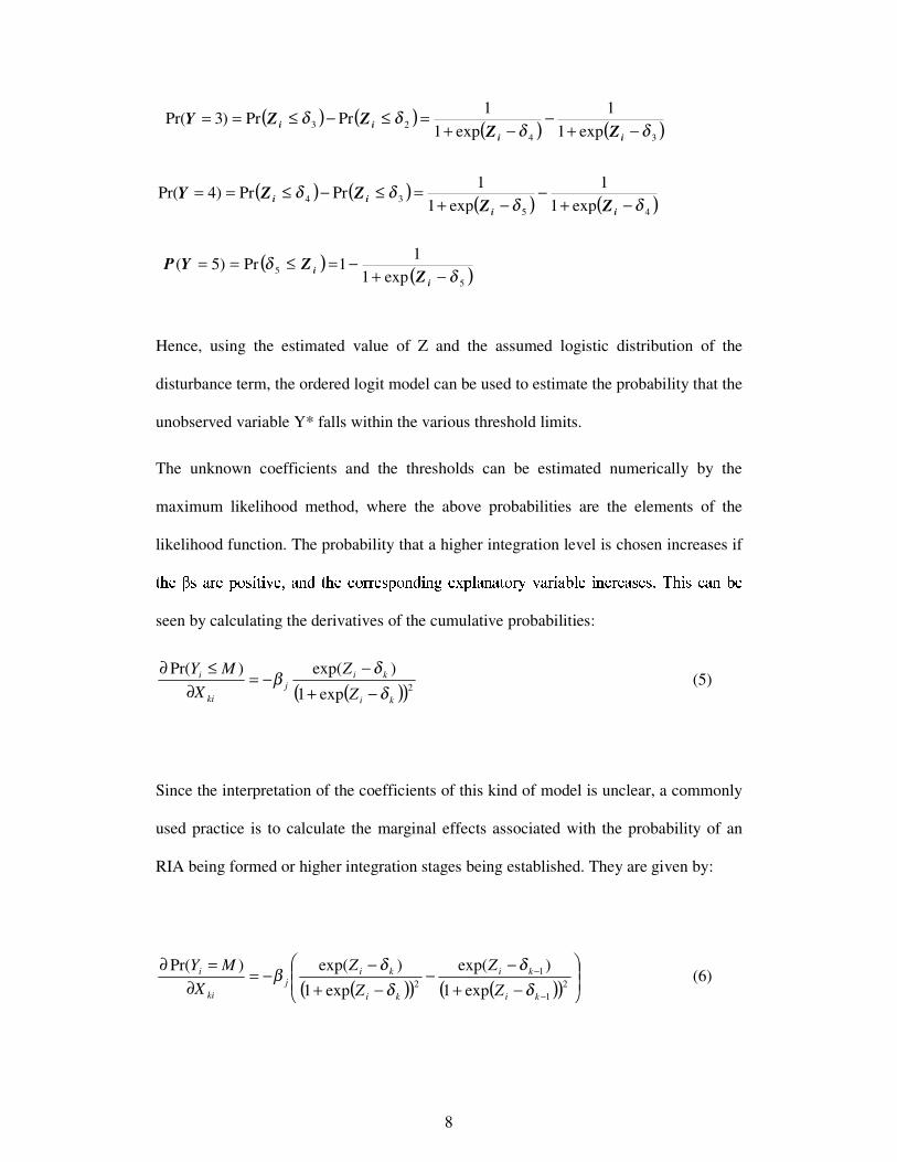
Hence, using the estimated value of Z and the assumed logistic distribution of the

disturbance term, the ordered logit model can be used to estimate the probability that the

unobserved variable Y* falls within the various threshold limits.

The unknown coefficients and the thresholds can be estimated numerically by the

maximum likelihood method, where the above probabilities are the elements of the

likelihood function. The probability that a higher integration level is chosen increases if

¯9°M±�² ³µ´N¶6· ¸M¹G³»º¦¼zº[½G·X¾i´5¿3À�¼9ÁM·ÃÂX¹J¶Z¶6·X³S¸M¹J¿3ÀGº[¿3Äq·NÅG¸MÆ9´x¿3´N¼z¹f¶|Ç�½G´5¶nº�´]ÈMÆ�·Ãº[¿MÂ5¶n·5´a³�·X³xÉËÊiÁuºv³1Â]´5¿ÌÈG·

seen by calculating the derivatives of the cumulative probabilities:

( )( )2exp1

)exp()Pr(

ki

kij

ki

i

Z

ZX

MY

δδ

β−+

−−=

∂≤∂

(5)

Since the interpretation of the coefficients of this kind of model is unclear, a commonly

used practice is to calculate the marginal effects associated with the probability of an

RIA being formed or higher integration stages being established. They are given by:

( )( ) ( )( )

−+−

−−+

−−=

∂=∂

−

−2

1

12 exp1

)exp(

exp1

)exp()Pr(

ki

ki

ki

kij

ki

i

Z

Z

Z

ZX

MY

δδ

δδβ (6)

( ) ( )55 exp1

11Pr)5(

δδ

−+−=≤==

ii Z

ZYP

9

An advantage of an ordered logit over an ordered probit model is its simplicity.

However, it is subject to the Independence of Irrelevant Alternatives (IIA) property,

which constitutes a tight limitation, as all alternatives must follow an independent

choice function. Selection pairs Pi/Pj of alternative i over j are independent on whether

third alternatives exist. The advantage of this condition is that it enables the introduction

of new alternatives –such as new integration levels- with no need to re-estimate the

model. The difference between the estimated parameters must be the same, regardless of

the number of alternatives the economic agent faces. The disadvantage of this property

is that alternatives must be perceived as distinct and independent.

The evaluation of this type of model differs in certain ways from traditional models.

Even though the ratio of an estimated coefficient to its corresponding estimated

standard error follows a t-Student distribution, the F test is not appropriate for these

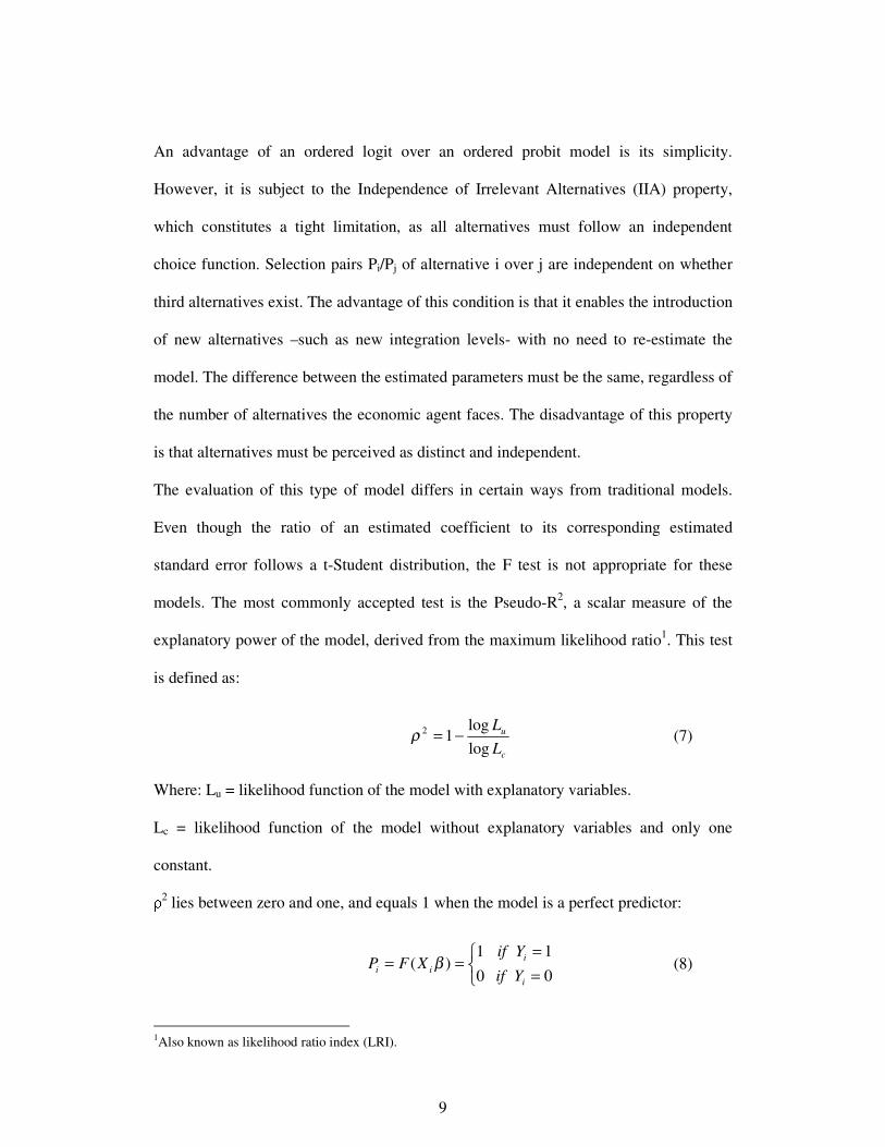
models. The most commonly accepted test is the Pseudo-R2, a scalar measure of the

explanatory power of the model, derived from the maximum likelihood ratio1. This test

is defined as:

c

u

LL

loglog

12 −=ρ (7)

Where: Lu = likelihood function of the model with explanatory variables.

Lc = likelihood function of the model without explanatory variables and only one

constant.

Í 2 lies between zero and one, and equals 1 when the model is a perfect predictor:

0

1

0

1)(

==

==i

iii Yif

YifXFP β (8)

1Also known as likelihood ratio index (LRI).

10

P takes value 0 if log Lc = log Lu, thus ρ2 increases to 1 when log Lc rises in relation to

log Lu.

An alternative way to evaluate the goodness of fit of an ordered logit is to calculate the

exp (log likelihood / number of observations) which is the geometric average of P (Oj /

Xj, estimates), where Oj and Xj are the outcome and the explanatory variables for

observation j. This ratio shows the probability of obtaining a certain outcome

conditional on the estimates. The higher the ratio is, the greater the explanatory power

of the model will be.

The interpretation of coefficients in an ordered logit model also differs explicitly from

other models. In discrete choice logit and probit models, the sign of the coefficients

denotes the direction of switch, but its magnitude is difficult to interpret. For example,

in the ordered logit model estimated in this paper, positive coefficients corresponding to

characteristics of the individuals increase the probability that a pair of countries will be

observed in a higher integration category, whereas negative coefficients increase the

probability that a pair of countries will be observed in a lower integration category.

3. Data, hypothesis and variables

3.1 The data

The model is estimated with 1999 data for 66 countries representing over 75% of world

trade (see Table A.1, Appendix A). Data on income are obtained from the World

Development Indicators (2001). Distances are the great circle distances between

economic centres. Data on capital labour ratios are obtained from the Penn World

Tables. Data on bilateral exports are obtained from Statistics Canada (2001), and tariff

barriers from the World Bank website. Information about geographical and language

dummies is from the CIA (2003). The Economic Freedom index was obtained from the

Heritage Foundation, and the political regime, from the Freedom House. Table A.2 in

11

Appendix A presents a more detailed description of data and sources. Finally, the

agreements considered to build the depended variable are listed in Table A.3 (Appendix

A).

3.2. Hypothesis and variables

According to the underlying theory described in Section 2 above and in the context of

the discrete choice model, our first hypothesis is that a pair of countries will be more

likely to form an RIA when the distance between them is small. We specify the distance

variable as in BB. This variable is called “natural” as it is defined as the logarithm of the

inverse of distance between trading partners.

A second hypothesis is that the probability of RIA formation increases as the

remoteness of a country or pair of countries from the rest of the world rises. For

comparative purposes, we construct the same remoteness variable used by BB. When a

country is relatively far from its trading partners, it tends to trade more bilaterally with

its neighbours, thereby increasing the probability of RIA formation.

The third hypothesis is that the larger the economic size of the trading countries, the

greater the probability of RIA formation will be. RGDPij measures the sum of the logs

of real GDPs of countries i and j in 19602.

The fourth hypothesis is that the more similar in economic size the countries are, the

higher the probability of RIA formation will be. DRGDPij is the absolute value of the

difference between the logs of real GDPs of countries i and j in 1960.

The fifth hypothesis is that the larger the economic size of countries outside the RIA,

the higher the probability of RIA formation will be. However, the size of the rest of the

world (ROW) measured by the ROW GDP varies only slightly in a cross-section of

2 Data are from 1960 to avoid problems derived from the endogeneity of income in the estimated equation. The same applies to the variables DRGDPij and DKLij .

12

countries and has not been included in the regression. BB obtained a non-significant

coefficient for this variable.

The sixth hypothesis is that the probability that a pair of countries will form an RIA is

higher if they have a larger difference in relative factor endowments, since traditional

comparative advantages will be further exploited. However, if intercontinental transport

costs are low, this probability may also decrease at high levels of specialisation. This

can be modelled by adding a quadratic term to the estimated equation. We use absolute

differences in the capital stock per worker ratio (DKLij) as a proxy for relative factor

endowment differences, as in BB3. SQDKLij denotes squared DKLij.

The first model estimated is a binary probit where the dependent variable takes the

value of one when the countries have an integration agreement, zero otherwise, and the

independent variables are those listed above.

The second model estimated is an ordered logit. Five possible different levels of

integration between pairs of countries are considered to investigate the determinants of

regional integration agreements (RIAs). In this context, supplementary economic,

geographical and socio-political variables are added as determinants of RIAs. Tariff

barriers and bilateral trade flows were initially added as economic variables. Trade

barriers were expected to have a negative sign, since a higher level of protection can be

an obstacle to a higher integration level being reached. Trade flows were expected to

have a positive sign, since more trade between countries indicates a strong relationship

and dependence and a reason to sign an RIA. However, due to the endogeneity

problems found for bilateral trade, we chose to exclude this variable from the

estimations. Magee (2003) provides one of the first assessments of the hypothesis that

two countries are more likely to form a PTA if they are already major trading partners.

3 Data are for 1965 rather than 1960, since data on capital labour ratios is only available from 1965 onwards in the Penn World Tables data series. Baier and Bergstrand (2004) use data for 1960.

13

He estimates a probit and a non-linear two-stage least squares model that considers

trade flows as endogenous in the second specification. Magee’s results show that in

every specification of the model, greater bilateral trade flows significantly increase the

likelihood that countries will form a preferential trade agreement.

Landlocked status and adjacency are added to the list of geographical variables used by

BB. Adjacency is expected to have a positive sign, whereas being landlocked could

have a positive or a negative sign. On the one hand, a landlocked country has greater

incentives to eliminate trade restrictions with neighbours, especially with non-

landlocked countries. On the other hand, when a landlocked country trades with partners

located in another continent (unnatural partner), it will have higher transport costs than a

coastal country.

Finally, the socio-political variables are: sharing a common language, the political

regime (this variable takes a value of 1 when the political regime is a democracy) and

the level of economic freedom. The economic freedom variable takes a value between

1-1.99 for free countries, 2-2.99 for mostly free countries, 3- 3.99 for mostly non-free

countries and 4-4.99 for repressed countries. Language and democracy dummies are

expected to have a positive sign, whereas economic freedom is expected to have

negative coefficients4.

4. Estimation Results

4.1 Probit estimation

The results obtained when a binary probit is estimated are shown in Table 1. The

results will be comparable to those obtained by BB5 although the sample of

4 Note that according to the definition of these variables, higher values imply lower economic freedom. 5 Table B.1 in Appendix B.

14

countries considered is not exactly the same, the year is 1999 instead of 1996,

and the definition of the dependent variable also varies slightly.

Table 1. Probit results for the probability of RIA formation or enhancement

The first hypothesis to be tested is that the smaller the distance between the two

countries, the more likely their social planners will be to form an RIA, since the closer

two trading partners are, the lower their trade barriers will be. The probability of

establishing an RIA increases with diminishing distances between the trading countries.

BB obtain a positive coefficient (1.74) in their equivalent Model 1. We also obtain a

positive coefficient (0.56), but it is lower in magnitude.

In Model 2, the second hypothesis is tested. For a given distance between two countries,

the more remote the two continental trading partners are from the rest of the world, the

more likely they will be to form an RIA. We calculate this variable according to BB and

we obtain a positive coefficient similar in magnitude.

In Model 3, the third hypothesis is that the larger the trading partners are in economic

terms, the greater the probability of an RIA being formed will be. This effect is captured

by RGDPij and it is positive and significant, as expected. However, the coefficient

obtained in this paper is lower than that obtained in BB.

In Model 4, the fourth hypothesis is tested. The greater the similarity between the

economic size of the two countries, the higher the probability of an RIA being

established will be. This effect is captured by DRGDPij. We obtain the expected

negative sign and this variable is significant.

Finally, the sixth hypothesis is tested in Models 5, 6 and 7. According to BB, the larger

the difference between countries’ relative factor endowments, the greater the probability

of FTA formation will be, although this may only be true to a limited extent. The

variables DKLij and SQDKLij (DKLij squared) measure this effect. When we include

15

these two variables in the same regression, they are not significant. Since the two

variables are highly correlated, DKLij and SQDKLij are included in Models 5 and 7

respectively. Both variables are significant, but they do not have the expected signs. The

negative sign obtained for DKLij indicates that the larger the difference between

countries’ relative factor endowments is, the lower the probability of an RIA will be.

This result indicates that the social planners from the two countries tend to form an RIA

when they have similar relative factor endowments. Accordingly, higher levels of intra-

industry trade will be desirable if RIAs are to be formed, since countries with similar

endowments trade similar commodities. This does not support the notion of “natural

trading partners” defined by Schiff (1999) as complementarities between partners (one

country tends to import what the other exports). A plausible explanation from the

demand side may be that because countries with similar endowments have similar tastes

and love variety, their governments will be more likely to negotiate higher levels of

integration.

BB test an additional hypothesis. The higher the absolute difference between the

relative factor endowment of the member countries and the relative factor endowment

of the rest of the world, the lower the probability of FTA formation will be, due to

potential trade diversion. We construct DROWKLij according to BB, although we

aggregate the ratio K/L rather than aggregating both variables separately6, since we do

not have detached data for capital and labour. We use equation (9) to calculate

DROWKLij.

6 Baier and Bergstrand (2004) measure DROWKLij as:

[ ] [ ]2

}loglogloglog{,1,1,1,1

jj

N

ikkk

N

jkkkii

N

ikkk

N

jkkk LKLKLKLK

DROWKLij

−

+−

=∑∑∑∑

≠=≠=≠=≠=

16

[ ] [ ] [ ] [ ]

2

}log/loglog/log{,1,1

jj

N

jkkkkii

N

ikkkk LKLKLKLK

DROWKLij

−

+−

=∑∑

≠=≠= (9)

The coefficient of this variable is close to zero (0.05) and is not significant.

Differences in the two sets of results can be explained by the different constructions of

the dependent variable: BB consider only full FTAs or customs unions, whereas our

dependent variable includes all PTAs, FTAs, CUs, SMs and MUs notified to

GATT/WTO under Article XXIV and under the Enabling Clause (see Table A.3,

Appendix A). This variable is broader since it regards integration agreements as a

process with different levels of integration; with this construction it make sense to

estimate an ordered logit.

BB use the Pseudo R2, calculated according to equation (7) above, as a measure of

explanatory power. However, Heinen (1993) points out that although this index is not

affected by changes in the sample size, it is affected by the presence of missing

observations. In this case, a better alternative is to calculate McFadden’s R2, which

takes the missing values into account. Table 1 shows both the Pseudo R2 and the

McFadden’s R2. The McFadden statistic considers that there is a different number of

observations in the restricted and unrestricted models when there are missing values for

some variables. In the estimated models 3-7, the McFadden’s R2 is preferred to the

Pseudo R2 since there are zero values in some of the explanatory variables.

4.2 Ordered logit estimation

We estimate an ordered logit model consisting of a system of 5 equations, with common

coefficients for all the explanatory variables and with different constant terms. This is

known as the proportional odds model.

17

In the first column of Table 2 (Model 8), an ordered logit is estimated with the same

variables included in Model 5 (probit estimation). Model 9 to Model 12 in columns 2 to

6 of Table 2 are estimated for different sets of variables grouped as economic,

geographical and socio-political variables. This sequential analysis enables us to find

out the most important factors in promoting RIAs.

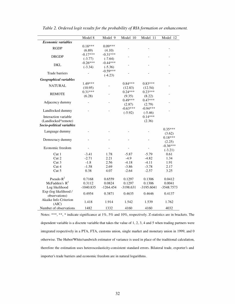
Table 2. Ordered logit results for the probability of RIA formation or enhancement

Model 8 shows that the results are similar in both probit and ordered logit models,

although the logit ordered coefficients are higher in magnitude. In general terms, we can

state that the probability of reaching a higher level of integration is higher than the

probability of signing any type of RIA when no previous agreement exists between the

trading countries. However, as stated above, there is no consensus on the interpretation

of the magnitude of the coefficients estimated in discrete choice models.

Model 9 shows the results obtained when only economic variables are included in the

analysis. The coefficient on tariffs is negative, thus showing that a higher level of

protection decreases the probability of RIA enhancement.

Models 10 and 11 in Table 2 show the results for the geographical variables. All

geographical variables are significant at 1%, and natural, remoteness and adjacency

have a positive signed coefficient, while the landlocked variable coefficient is negative.

In Model 11 the interaction variable (landlocked*remoteness) is added to consider the

ambiguous sign expected for the landlocked variable. The estimated coefficient shows a

positive sign, indicating that the probability of reaching a higher level of integration

increases for more remote continental trading partners when one of them is landlocked.

18

Model 12, in the last column of Table 2, shows that all the socio-political variables are

significant: democracy, the level of economic freedom and the common language

promote RIA enhancement. However, in terms of goodness of fit, the Pseudo R2 is very

low (0.04).

The AIC shows that the best specification is the one estimated in Model 8, where

economic and geographical variables are considered. For the specification where only

geographical variables are considered, the AIC is lower (1.542) than that obtained in

regressions including only economic (1.914) or only socio-political factors (1.762). This

appears to indicate that geographical variables are the most important determinants of

RIA formation.

We would have preferred the ideal specification of the model to simultaneously include

all the significant variables: economic, geographical and socio-political variables.

However, problems related to the correlation between the explanatory variables

prevented us from doing this.

As stated above, the interpretation of the coefficients in an ordered logit does not inform

on the magnitude of switch, since we can only state that positive coefficients increase

the likelihood that the country pairs will be observed in a higher category, and negative

coefficients increase the likelihood the country pairs will be observed in a lower

category. A preferable interpretation of the ordered logit coefficients is in terms of the

odd ratios. The exponentiated coefficients in logit, shown in Table 3, can be interpreted

as odds ratios for a 1-unit change in the corresponding variable. The emphasis is on the

ratio “Exp(β)”, which is the odds conditional on x+1 divided by the odds conditional on

x. For example, 1.19 means that the odds of being in a higher integration level increase

1.19 if RGDP increases by 1. The interpretation can also be made in terms of

percentages: the exp(1.49) obtained in the “natural” variable in Model 8 means the odds

19

increase by 346% {[exp(1.49)-1]*100} if the variable increases by 1, therefore the

odds of being part of the monetary union versus lower integration levels is 346% higher

for a one-unit increase in the “natural” variable. Table 3 shows that the most important

determinant of an RIA is the “natural” variable, followed by remoteness (1.37), real

GDP (1.19), real GDP differences (0.84) and K/L differences (0.77).

We also calculate semi-standardised ordered logit coefficients that control for the metric

of the independent variables, to see whether any change occurs in the ordering of the

effects. The option of standardised coefficients to measure the relative strength of the

effects of the independent variables is more appropriate in the current empirical

application, since some of the independent variables are measured in different units.

Table 3 shows that when standardised coefficients are considered (e^bStdX), the

ordering of the effects changes only slightly. In Model 8, the natural variable

standardised coefficient is 3.89, for remoteness it is 1.76, for RGDP it is 1.65, for K/L

differences 0.75, and for real GDP differences 0.74. For one standard deviation increase

in “natural”, the odds are 3.89 times greater (an increase of 289%) of countries being in

a higher integration category, when all other variables are held constant.

Table 3. Odds ratios for the ordered logit.

In order to evaluate the probability that the dependent variable will have a particular

value, we use cut-offs terms. From equation (1) the threshold parameters for Model 8

are given by:

Yi = 0 if Y*i Î -3.41

Yi = 1 if –3.41 Î Ï Ð i Î -2.71

Yi = 2 if –2.71 Î Ï Ð i Î -1.8

20

Yi = 3 if –1.8 Ñ Ò$Ó i Ñ -1.58

Yi = 4 if –1.58 Ñ Ò Ó i ÔÖÕM×ÙØMÚ

Yi = 5 if Y*i Û�Õu×ÜØMÚ

For example, when the trading partners are Argentina and Paraguay, we can calculate

the probability associated with this pair of countries by computing Zi with the obtained

coefficients in Model 8 and the correspondent data:

28.2)98.331.0())94.6(49.1()3.326.0()22.417.0()7.4618.0(54321

−=⋅+−⋅+⋅−+⋅−+⋅==⋅+⋅+⋅+⋅+⋅= NATURALREMOTEDKLijDRGDPijRGDPijZ i βββββ

( ) ( ) 2442.0)41.3(28.2exp1

10Pr)0Pr( =

−−−+=≤== iZY

( ) ( ) ( ) ( ) 1499.0)41.3(28.2exp1

1)71.2(28.2exp1

10PrPr)1Pr( 1 =

−−+−

−−−+=≤−≤== ii ZZY δ

( ) ( ) ( ) ( ) 2236.0)71.2(28.2exp1

1)8.1(28.2exp1

1PrPr)2Pr( 12 =

−−−+−

−−−+=≤−≤== δδ ii ZZY

( ) ( ) ( ) ( ) 0505.0)8.1(28.2exp1

1)58.1(28.2exp1

1PrPr)3Pr( 23 =

−−−+−

−−−+==≤−≤== δδ ii ZZY

( ) ( ) ( ) ( ) 2664.0)58.1(28.2exp1

1)38.0(28.2exp1

1PrPr)4Pr( 34 =

−−−+−

−−+=≤−≤== δδ ii ZZY

( ) ( ) 0654.0)38.0(28.2exp1

11Pr)5( 5 =

−−+−=≤== iZYP δ

Hence, for Argentina and Paraguay the most likely outcome is that they will form a

single market. In fact, they have been members of Mercosur since 1995.

Our second example is Spain and France, a pair of trading partners that are members of

the European Union. Our results indicate that the highest probability is that of the

establishment of a single market. In 1999 these countries were already in the third phase

of the European Monetary Union (EMU), since they fulfilled the convergence criteria

established in the Treaty of Maastricht. However, our results most probably show that

they were only in the EMU starting phase.

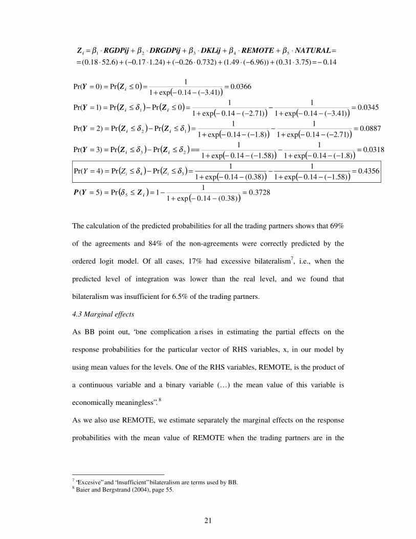
21

14.0)75.331.0())96.6(49.1()732.026.0()24.117.0()6.5218.0(54321

−=⋅+−⋅+⋅−+⋅−+⋅==⋅+⋅+⋅+⋅+⋅= NATURALREMOTEDKLijDRGDPijRGDPijZ i βββββ

( ) ( ) 0366.0)41.3(14.0exp1

10Pr)0Pr( =

−−−+=≤== iZY

( ) ( ) ( ) ( ) 0345.0)41.3(14.0exp1

1)71.2(14.0exp1

10PrPr)1Pr( 1 =

−−−+−

−−−+=≤−≤== ii ZZY δ

( ) ( ) ( ) ( ) 0887.0)71.2(14.0exp1

1)8.1(14.0exp1

1PrPr)2Pr( 12 =

−−−+−

−−−+=≤−≤== δδ ii ZZY

( ) ( ) ( ) ( ) 0318.0)8.1(14.0exp1

1)58.1(14.0exp1

1PrPr)3Pr( 23 =

−−−+−

−−−+==≤−≤== δδ ii ZZY

( ) ( ) ( ) ( ) 4356.0)58.1(14.0exp1

1)38.0(14.0exp1

1PrPr)4Pr( 34 =

−−−+−

−−+=≤−≤== δδ ii ZZY

( ) ( ) 3728.0)38.0(14.0exp1

11Pr)5( 5 =

−−+−=≤== iZYP δ

The calculation of the predicted probabilities for all the trading partners shows that 69%

of the agreements and 84% of the non-agreements were correctly predicted by the

ordered logit model. Of all cases, 17% had excessive bilateralism7, i.e., when the

predicted level of integration was lower than the real level, and we found that

bilateralism was insufficient for 6.5% of the trading partners.

4.3 Marginal effects

As BB point out, “one complication a rises in estimating the partial effects on the

response probabilities for the particular vector of RHS variables, x, in our model by

using mean values for the levels. One of the RHS variables, REMOTE, is the product of

a continuous variable and a binary variable (…) the mean value of this variable is

economically meaningless”. 8

As we also use REMOTE, we estimate separately the marginal effects on the response

probabilities with the mean value of REMOTE when the trading partners are in the

7 “Excesive” and “insufficient” bilateralism are terms used by BB. 8 Baier and Bergstrand (2004), page 55.

22

same continent, and when REMOTE takes the value of zero (the trading partners are

not in the same continent, they are unnatural partners).

Marginal effects are calculated for Model 5 (probit) and Model 8 (ordered logit). Our

results for the probit estimation are shown in Table 4 and for the ordered logit

estimation in Table 5. Our results in Table 4 can be compared with those obtained by

BB, shown in Appendix B (Tables B.1 and B.2).

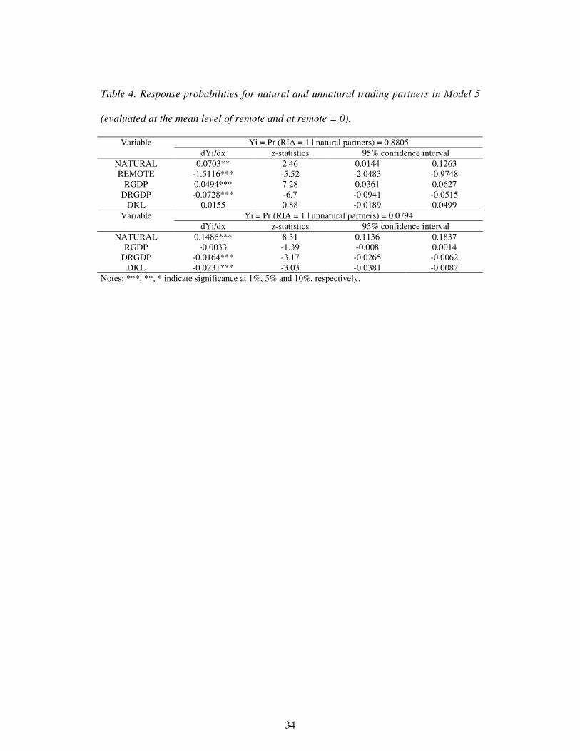
Table 4. Response probabilities for natural and unnatural trading partners in Model 5

(evaluated at the mean level of remote and at remote = 0).

Table 4 shows that the response probability of an RIA being created is much lower for

unnatural partners (7.94%) than for natural partners (88.05%). Moreover, results show

that a unitary increase in proximity (natural variable) increases this probability by

7.03% for two natural partners and 14.86% for unnatural partners. An increase in

remoteness from the rest of the world of two natural partners lessens the response

probability in natural partners. Although this is an unexpected result, Table 5 shows that

the sign of this marginal effect changes for different levels of integration when the

model estimated is an ordered logit rather than a binary probit model. This sign is only

positive for the first two integration stages (PTA and FTA). When two countries are in

the same continent and they are relatively far away from the other countries in this

continent, then the probability that they will reach a customs union decreases with the

level of remoteness.

Results also show that economic variables have a lower effect than geographical factors

on response probabilities, although differences in income also play an important role in

RIA creation.

23

The response probability for natural partners is similar to that obtained by BB, who

find 86.7% probability of a FTA being established between natural partners. However,

they only obtain a probability of 1.2% for unnatural partners. We obtain a higher

probability for unnatural partners because we also considered preferential trade

agreements in the construction of the dependent variable.

To compare the effect of the RHS variables across different levels of integration, in

Table 5 we estimate the marginal effects for all the integration levels for both natural

and unnatural partners.

Table 5. Response probabilities for natural and unnatural trading partners in Model 8

(evaluated at the mean level of remote and at remote = 0).

Table 5 shows different probabilities depending on the level of integration. For each

level of integration, the probabilities are shown for natural and for unnatural partners.

However, for the three last categories (customs union, single market and monetary

union) the probabilities can only be calculated for natural partners, since these

integration levels are only reached by countries in the same continent. These

probabilities depend mainly on geographical and economic variables, and their marginal

effects differ across integration levels.

On the one hand, the results obtained for natural partners (countries in the same

continent) indicate that when remoteness increases by 1%, the probability of a PTA or

an FTA being established increases by 199% and 57% respectively. However, the

probability of a customs union or a higher integration agreement being established

decreases with remoteness. This variable, together with real GDP, is the most influential

factor on the probability of an RIA being formed or enhanced between natural partners.

24

Higher GDP differences increase the probability of PTA or FTA formation for natural

partners, although for higher levels of integration, the sign of the marginal effect is

reversed, thus indicating that similarity of income, as expected, increases the probability

that higher levels of integration (customs union, single market and monetary union) will

be reached. Integration theory predicts that the costs of integration are lower when the

countries have similar income levels and consequently, a high level of intra-industry

trade.

On the other hand, for unnatural partners (countries in a different continent) the inverse

of distance is the most important factor in PTA or FTA formation and higher

differences in income and in factor endowments lower the probability of a PTA or an

FTA being established.

According to our results, the most likely outcomes are that natural partners will

establish a single market and unnatural partners will not establish any agreement.

4.3 Sensitivity Analysis

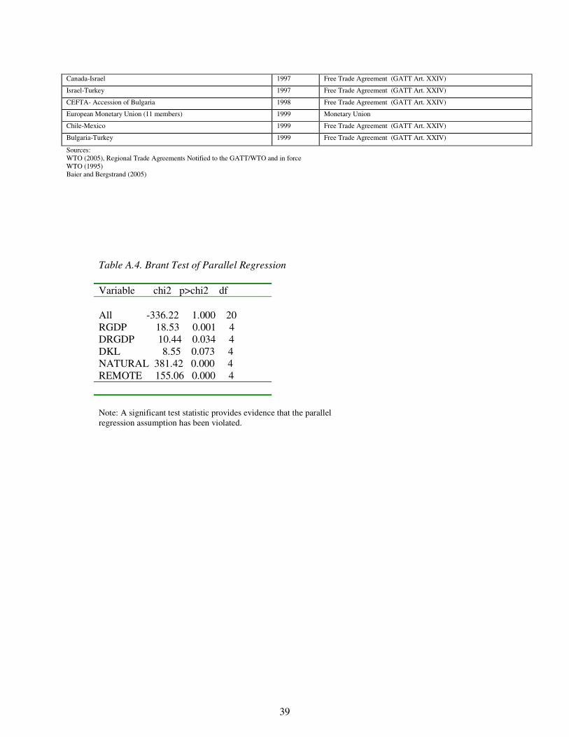
We performed several robustness tests to validate our results. First, the ordered logit

model is based on the assumption of parallel slopes but this may be unrealistic, for

example if geographical variables are less relevant for higher integration levels.

Therefore, the brant test of the parallel regression assumption is used to validate the

methodology used. The Brant (1990) test assesses whether or not the coefficients are the

same for each category of the dependent variable. This produces Wald Tests for the null

hypothesis that the coefficients in each independent variable are constant across

categories of the dependent variable. Significant test statistics provide evidence that this

assumption has been violated for most of the variables. With the exception of the

capital-labour ratio, we cannot accept the equality of slopes for the different levels of

integration (Table A.4). These results indicate that we should estimate a generalised

25

logit model, and they suggest what variables may be used in determining the

thresholds. We therefore estimated a generalised ordered logit for all the regressions

presented in Table 2. In some cases, the model did not converge, especially when the

variables with missing data (K-L differences) were included. The results9 indicate that

the geographical variables are significant and show the expected signs for the lower

levels of integration (PTA, FTA), whereas for the higher levels these variables lose

significance and decrease in magnitude. In contrast, the economic and political variables

gain importance in the higher levels of integration.

Secondly, we re-estimated the probit and ordered logit model with an alternative data

set taken from Magee (2003), which are available for replications on the webside. His

dependent variable takes the value of one if the country pair has a PTA in 1998 and zero

otherwise. We use the same dependent variable in the probit estimation, but Magee

(2003) considers fewer agreements since they ignore the General System of Trade

Preferences (GSTP), the Protocol related to Trade Negotiations among developing

countries (PTN) and the African Common Market. Additionally, the variable

remoteness is not included as explanatory variable in Magee (2003). We estimate a

binary probit for 172 countries in 1998 and our results confirm the sign and significance

of the estimated coefficients for the income variables, the relative factor endowment

differences and the natural variable (Model 7.1 in Table 1). Contrary to BB, the K-L

differences variable is negative and significant, thus validating our evidence. Similar

results are obtained when an ordered logit is estimated.

Thirdly, we also estimated the probit model with the inclusion of bilateral trade as an

explanatory variable and using instrumental variables to correct for endogeneity

problems. Infrastructure variables were used as instruments for trade. The results

9 Results are not shown for reasons of space, but are available from the authors upon request.

26

indicate that trade is significant and has a positive sign when it is added to the list of

explanatory variables in the probit model, confirming the evidence presented by Magee

(2003) with different data and different model specifications. However, as stated above

further research is needed to solve problems related to the high correlation among the

independent variables and to improve the model specification.

Finally, the ordered nature of the dependent variable and the endogeneity of trade flows

should ideally be considered simultaneously, but this is beyond the scope of this

research.

5. Conclusions

In this paper, discrete choice modelling is used to study the determinants of regional

trade agreements. A binary probit model and an ordered logit model are estimated, in

which geographical, economic and socio-political variables are considered as

explanatory variables for RIA formation. Five different integration levels are specified

for the dependent variable in the ordered logit estimation.

The results from the probit and ordered logit estimations show that the probability of

reaching a higher level of integration increases with income level, economic freedom,

cultural affinities and remoteness, whereas it decreases with distance, protection levels,

income differences and factor endowment differences. Additionally, geographical

variables seem to be the most important determinants of RIA formation.

The marginal effects, calculated for natural and unnatural trading partners, show that

countries in the same continent (natural partners) will most probably establish a single

market, whereas countries in different continents (unnatural partners) are most likely not

to sign any agreement. This result is new in the RIA literature and should be validated

by extending the sample to include more years and countries. The marginal effects also

show that some variables, such as remoteness and differences in real GDP, have a

27

positive influence on the formation of an RIA, but only for countries in the same

continent and in the early stages of the integration process (PTA, FTA). However, when

the categories considered are higher integration levels, the effect of these two variables

is reversed.

The estimation of a trade equation that considers the formation of RIAs as an

endogenously determined explanatory variable remains an issue for further research.

The extension of the sample to include more years would enable dynamic issues to be

analysed.

28

References

Akiva, and Lerman (1985) Discrete Choice Analysis. Theory and Application to Travel

Demand. The MIT Press.

Amemiya, T. (1975): Qualitative Response Models. Ann. Econ. Social Measurement 4,

363-372.

Baier, S.L. and Bergstrand, J.H. (2004): Economic Determinants of Free Trade

Agreements. Journal of International Economics 64 (1), 29-63.

Baier, S.L. and Bergstrand, J.H (2005): Do free trade agreements actually increase

members’ international trade?, Working Paper 2005 -03, Federal Reserve Bank

of Atlanta.

Ben-Akiva, M., and Lerman, S. (1985): Discrete Choice Analysis. MIT Press,

Cambridge, Massachusetts.

Brant, R. (1990): Assessing Proportionality in the Proportional Odds Model for Ordinal

Logistic Regression. Biometrics 46, 1171-1178.

Central Intelligence Agency –CIA– (2003): The World Factbook. From

http://www.odci.gov/cia/publications/factbook

Frankel, J.A., Stein, E. and Wei, S.-J. (1995): Trading Blocs and the Americas: the

natural, the unnatural, and the super-natural. Journal of Development Economics

47 (1), 61–95.

Frankel, J.A., Stein, E. and Wei, S.-J. (1996): Regional trading arrangements: natural or

supernatural. American Economic Review 86 (2), 52–56.

Frankel, J.A., Stein, E. and Wei, S.-J. (1998): Continental trading blocs: are they natural

or supernatural. In: Frankel, J.A., Editor, , 1998. The Regionalization of the

World Economy, University of Chicago Press, Chicago, 91–113.

Great circle distances (2003): From http://www.wcrl.ars.usda.gov/cec/java/lat-long.htm

29

Heinen, T. (1993): Discrete Latent Variable Models. Tilburg University Press. The

Netherlands.

Koppelman, F.S. and Wen, C.(1998): Alternative nested logit models: Structure,

properties and estimation. Transportation Research 32 (3), 289-298.

Magee, C. (2003): Endogenous preferential trade agreements: An empirical analysis.

Contributions to Economic Analysis & Policy 2 (1), 1-17.

McFadden, D. and Train, K. (2000): Mixed MNL models for discrete response. Journal

of Applied Econometrics 15 (5), 447-470.

Miles, M. A., Feulner Jr., E. J., O’Grady M. A. a nd Eiras A. I (2004): Index of

Economic Freedom. The Heritage Foundation.

Penn World Tables (2005): From http://datacentre.chass.utoronto.ca/pwt56/

Schiff, M. (1999), “Will the Real “Natural Tradi ng Partner” Please Stand Up?” World

Bank, Development Research Department Working Paper.

Statistics Canada (2001): World Trade Analyzer. The International Trade Division of

Statistics of Canada.

The Freedom House (2005): Democracy’s Century. A Survey of Gl obal Political

Change in the 20th Century. From http://www.freedomhouse.org/

Viner, J., (1950): The Customs Union Issue, Carnegie Endowment for International

Peace, New York.

World Bank (2001): World Development Indicators, Washington.

World Bank (2005): From http://www.worldbank.org/

World Trade Organization (1995): Regionalism and the World Trading System. Geneva.

World Trade Organization (2005): From http://www.wto.org/

30

Wu, J. P.(2004): Measuring and explaining levels of regional economic integration.

Working Paper B12/2004. Centre for European Integration Studies. From

http://www.zei.de/

31

Table 1. Probit results for the probability of RIA formation or enhancement

Model 1 Model 2 Model 3 Model 4 Model 5 Model 6 Model 7 Model 7.1a

Constant 4.07*** (17.31)

2.07*** (6.34)

2.31*** (3.42)

1.63** (2.41)

2.35* (1.88)

2.32* (1.87)

2.34* (1.88)

-0.78 (-1.03)

NATURAL 0.56*** (20.3)

0.35*** (9.55)

0.56*** (11.37)

0.54*** (10.64)

0.85*** (8.51)

0.85*** (8.53)

0.86*** (8.51)

1.19*** (32.63)

REMOTE - 0.16*** (9.35)

0.14*** (6.65)

0.14*** (6.64)

0.16*** (4.40)

0.16*** (4.44)

0.16*** (4.32)

-

RGDP - - 0.04*** (3.81)

0.06*** (5.75)

0.09*** (6.4)

0.09*** (6.47)

0.09*** (6.44)

0.11*** (13.87)

DRGDP - - - -0.16*** (-9.47)

-0.15*** (-5.75)

-0.15*** (-5.83)

-0.15*** (-5.71)

-0.065*** (-3.47)

DKL - - - - -0.09** (-2.12)

-0.16 (-1.38) - -0.17***

(-6.99)

SQDKL - - - - - 0.02 (0.62)

-0.02* (-1.71)

-

Pseudo R2 0.1226 0.1418 0.4536 0.4696 0.7797 0.7798 0.7794 0.865 McFadden’s R 2 0.1226 0.1418 0.2087 0.2319 0.4289 0.429 0.4282 0.462 Log Likelihood -2014.167 -1969.952 -1254.244 -1217.419 -505.633 -505.485 -506.251 -1304

Number of observations 4160 4160 2756 2756 1482 1482 1482 9045

Notes: ***, **, * indicate significance at 1%, 5% and 10%, respectively. Z-statistics are in brackets. The dependent variable is a binary discrete variable that takes the value of 1 when trading partners were integrated in a PTA, FTA, customs union, single market and monetary union in 1999, and 0 otherwise. The Huber/White/sandwich estimator of variance is used in place of the traditional calculation, therefore the estimation uses heteroscedasticity-consistent standard errors. a Model 7.1 was estimated with an alternative data set for a cross-section of 172 countries in 1998 from Magee (2003).

32

Table 2. Ordered logit results for the probability of RIA formation or enhancement.

Model 8 Model 9 Model 10 Model 11 Model 12 Economic variables

RGDP 0.18*** (6.89)

0.09*** (4.10) - - -

DRGDP -0.17*** (-3.77)

-0.31*** (-7.64) - - -

DKL -0.26*** (-3.34)

-0.44*** (-5.36) - - -

Trade barriers - -0.59*** (-4.23) - - -

Geographical variables

NATURAL 1.49*** (10.95) - 0.84***

(12.83) 0.83*** (12.54) -

REMOTE 0.31*** (6.28) - 0.24***

(9.35) 0.23*** (8.22) -

Adjacency dummy - - 0.49*** (2.87)

0.47*** (2.79) -

Landlocked dummy - - -0.63*** (-5.92)

-0.94*** (-5.46) -

Interaction variable (Landlocked*remote) 0.14***

(2.36)

Socio-political variables

Language dummy - - - - 0.35*** (3.62)

Democracy dummy - - - - 0.18*** (2.25)

Economic freedom - - - - -0.36*** (-3.21)

Cut 1 -3.41 1.78 -5.87 -5.79 0.61 Cut 2 -2.71 2.21 -4.9 -4.82 1.34 Cut 3 -1.8 2.56 -4.18 -4.11 1.91 Cut 4 -1.58 2.69 -3.86 -3.78 2.17 Cut 5 0.38 4.07 -2.64 -2.57 3.25

Pseudo R2 0.7168 0.6559 0.1297 0.1306 0.0412

McFadden’s R2 0.3112 0.0824 0.1297 0.1306 0.0041 Log likelihood -1040.835 -1264.454 -3198.631 -3195.6041 -3548.7573

Exp (log likelihood / observations) 0.4954 0.3871 0.4635 0.4646 0.4137

Akaike Info Criterion (AIC) 1.418 1.914 1.542 1.539 1.762

Number of observations 1482 1332 4160 4160 4032

Notes: ***, **, * indicate significance at 1%, 5% and 10%, respectively. Z-statistics are in brackets. The

dependent variable is a discrete variable that takes the value of 1, 2, 3, 4 and 5 when trading partners were

integrated respectively in a PTA, FTA, customs union, single market and monetary union in 1999, and 0

otherwise. The Huber/White/sandwich estimator of variance is used in place of the traditional calculation,

therefore the estimation uses heteroscedasticity-consistent standard errors. Bilateral trade, exporter’s and

importer’s trade barriers and economic freedom are in natural logarithms.

33

Table 3. Odds ratios for the ordered logit.

Model 8 Model 9 Model 10

Model 11

Model 12

Economic variables coef 0.18*** 0.09*** - - - e^b 1.19 1.1 - - -

RGDP

e^bStdX 1.65 1.31 - coef -0.17*** -0.31*** - - - e^b 0.84 0.73 -

DRGDP

e^bStdX 0.74 0.59 - coef -0.26*** -0.44*** - - - e^b 0.77 0.64 - - -

DKL

e^bStdX 0.75 0.62 - coef - -0.59*** - - - e^b - 0.55 - - -

Trade barriers

e^bStdX - 0.64 - Geographical variables

coef 1.49*** - 0.84*** - - e^b 4.46 - 2.33 2.30 -

NATURAL

e^bStdX 3.89 - 2.10 2.08 coef 0.31*** - 0.24*** - - e^b 1.37 - 1.28 1.25 -

REMOTE

e^bStdX 1.76 - 1.51 1.47 coef - - 0.49*** - - e^b - - 1.63 1.60 -

Adjacency dummy

e^bStdX - - 1.09 1.09 coef - - -0.63*** 0.14*** - e^b - - 0.53 0.39 -

Landlocked dummy

e^bStdX - - 0.77 0.68 coef - - - 0.14*** - e^b - - - 1.15 -

Interaction variable (landlocked*remote)

e^bStdX - - - 1.14 Socio-political variables

coef - - - - 0.35*** e^b - - - - 1.41

Language dummy

e^bStdX - - - - 1.13 coef - - - - 0.18*** e^b - - - - 1.19

Democracy dummy

e^bStdX - - - - 1.09 coef - - - - -0.36*** e^b - - - - 0.70

Economic freedom

e^bStdX - - - - 0.88 Notes: ***, **, * indicate significance at 1%, 5% and 10%, respectively. Odd ratios are e^b and e^bstdX. e^b = exp(b) = factor change in odds for unit increase in X; e^bStdX = exp(b*SD of X) = change in odds for SD increase in X. The dependent variable is a discrete variable that takes the value of 1, 2, 3, 4 and 5 when trading partners were integrated respectively in a PTA, FTA, customs union, single market and monetary union in 1999, and 0 otherwise. The Huber/White/sandwich estimator of variance is used in place of the traditional calculation, therefore the estimation uses heteroscedasticity-consistent standard errors. Exporter’s and importer’s trade barriers and economic freedom are in natural logarithms.

34

Table 4. Response probabilities for natural and unnatural trading partners in Model 5

(evaluated at the mean level of remote and at remote = 0).

Variable Yi = Pr (RIA = 1 | natural partners) = 0.8805 dYi/dx z-statistics 95% confidence interval

NATURAL 0.0703** 2.46 0.0144 0.1263 REMOTE -1.5116*** -5.52 -2.0483 -0.9748

RGDP 0.0494*** 7.28 0.0361 0.0627 DRGDP -0.0728*** -6.7 -0.0941 -0.0515

DKL 0.0155 0.88 -0.0189 0.0499 Variable Yi = Pr (RIA = 1 | unnatural partners) = 0.0794

dYi/dx z-statistics 95% confidence interval NATURAL 0.1486*** 8.31 0.1136 0.1837

RGDP -0.0033 -1.39 -0.008 0.0014 DRGDP -0.0164*** -3.17 -0.0265 -0.0062

DKL -0.0231*** -3.03 -0.0381 -0.0082 Notes: ***, **, * indicate significance at 1%, 5% and 10%, respectively.

35

Table 5. Response probabilities for natural and unnatural trading partners in Model 8

(evaluated at the mean level of remote and at remote = 0).

Variable Yi = Pr (RIA = Preferential Trade Agreement | natural partners) = 0.1913 dYi/dx z-statistics 95% confidence interval

NATURAL -0.0093 -0.49 -0.0467 0.0281 REMOTE 1.9932*** 7.1 1.4431 2.5434

RGDP -0.0151*** -3.3 -0.024 -0.0061 DRGDP 0.0267*** 3.9 0.0133 0.0402

DKL 0.0225 1.43 -0.0084 0.0534 Variable Yi = Pr (RIA= Preferential Trade Agreement |unnatural partners) = 0.0367

dYi/dx z-statistics 95% confidence interval NATURAL 0.0913*** 8.45 0.0701 0.1125

RGDP -0.0016 -1.57 -0.0035 0.0004 DRGDP -0.0059** -2.41 -0.0109 -0.0011

DKL -0.0151*** -4.33 -0.0219 -0.0083 Variable Yi = Pr (RIA = Free Trade Agreement | natural partners) = 0.1832

dYi/dx z-statistics 95% confidence interval NATURAL -0.0027 -0.45 -0.0142 0.0088 REMOTE 0.5727*** 2.97 0.1942 0.9513

RGDP -0.0043** -2.37 -0.0079 -0.0007 DRGDP 0.0077** 2.51 0.0017 0.0137

DKL 0.0065 1.39 -0.0027 0.0156 Variable Yi = Pr (RIA = Free Trade Agreement | unnatural partners) = 0.0301

dYi/dx z-statistics 95% confidence interval NATURAL 0.0804*** 9.49 0.0638 0.0971

RGDP -0.0014 -1.62 -0.0031 0.0003 DRGDP -0.0053*** -2.75 -0.0091 -0.0015

DKL -0.0133*** -4.38 -0.0192 -0.0073 Variable Yi = Pr (RIA = Customs Union | natural partners) = 0.0991

dYi/dx z-statistics 95% confidence interval NATURAL 0.0011 0.52 -0.0029 0.0052 REMOTE -0.2349* -1.88 -0.4799 0.0101

RGDP 0.0018* 1.82 -0.0001 0.0037 DRGDP -0.0031* -1.77 -0.0066 0.0003

DKL -0.0026 -0.97 -0.008 0.0027 Variable Yi = Pr (RIA = Single Market | natural partners) = 0.3456

dYi/dx z-statistics 95% confidence interval NATURAL 0.0178 0.49 -0.0538 0.0894 REMOTE -3.8125*** -10.53 -4.5219 -3.103

RGDP 0.0288*** 3.6 0.0131 0.0445 DRGDP -0.0512*** -4.44 -0.0738 -0.0286

DKL -0.0431 -1.45 -0.1011 0.015 Variable Yi = Pr (RIA = Monetary Union | natural partners) = 0.0439

dYi/dx z-statistics 95% confidence interval NATURAL 0.0038 0.48 -0.0117 0.0193 REMOTE -0.8184*** -7.14 -1.0431 -0.5937

RGDP 0.0062*** 3.47 0.0027 0.0097 DRGDP -0.0109*** -4.22 -0.0161 -0.0059

DKL -0.0092 -1.51 -0.0212 0.0027

Notes: ***, **, * indicate significance at 1%, 5% and 10%, respectively.

36

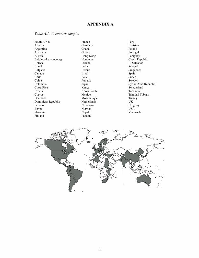
APPENDIX A

Table A.1. 66 country-sample.

South Africa Algeria Argentina Australia Austria Belgium-Luxembourg Bolivia Brazil Bulgaria Canada Chile China Colombia Costa Rica Croatia Cyprus Denmark Dominican Republic Ecuador Egypt Slovakia Finland

France Germany Ghana Greece Hong Kong Honduras Iceland India Ireland Israel Italy Jamaica Japan Kenya Korea South Mexico Mozambique Netherlands Nicaragua Norway Nepal Panama

Peru Pakistan Poland Portugal Paraguay Czech Republic El Salvador Senegal Singapore Spain Sudan Sweden Syrian Arab Republic Switzerland Tanzania Trinidad Tobago Turkey UK Uruguay USA Venezuela

37

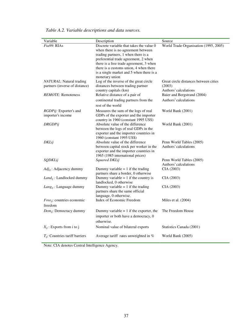
Table A.2. Variable descriptions and data sources.

Variable Description Source Fta99: RIAs Discrete variable that takes the value 0

when there is no agreement between trading partners, 1 when there is a preferential trade agreement, 2 when there is a free trade agreement, 3 when there is a customs union, 4 when there is a single market and 5 when there is a monetary union

World Trade Organisation (1995, 2005)

NATURAL: Natural trading partners (inverse of distance)

Log of the inverse of the great circle distances between trading partner country capitals (km)

Great circle distances between cities (2003) Authors’ calculations

REMOTE: Remoteness Relative distance of a pair of continental trading partners from the rest of the world

Baier and Bergstrand (2004) Authors’ calculations

RGDPij: Exporter’s and importer’s income

Measures the sum of the logs of real GDPs of the exporter and the importer country in 1960 (constant 1995 US$)

World Bank (2001)

DRGDPij Absolute value of the difference between the logs of real GDPs in the exporter and the importer countries in 1960 (constant 1995 US$)

World Bank (2001)

DKLij Absolute value of the difference between capital stock per worker in the exporter and the importer countries in 1965 (1985 international prices)

Penn World Tables (2005) Authors’ calculations

SQDKLij Squared DKLij Penn World Tables (2005) Authors’ calculations

Adjij : Adjacency dummy Dummy variable = 1 if the trading partners share a border, 0 otherwise

CIA (2003)

Landij : Landlocked dummy Dummy variable = 1 if the country is landlocked, 0 otherwise

CIA (2003)

Langij : Language dummy Dummy variable = 1 if the trading partners share the same official language, 0 otherwise.

CIA (2003)

Freeij: countries economic freedom

Index of Economic Freedom Miles et al. (2004)

Demij: Democracy dummy Dummy variable = 1 if the exporter, the importer or both have a democracy, 0 otherwise.

The Freedom House

Xij : Exports from i to j

Nominal value of bilateral exports Statistics Canada (2001)

Tij: Countries tariff barriers

Average tariff rates unweighted in % World Bank (2005)

Note: CIA denotes Central Intelligence Agency.

38

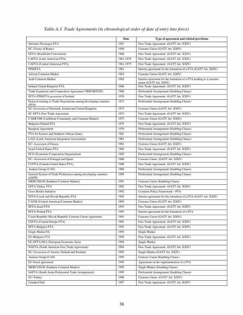
Table A.3. Trade Agreements (in chronological order of date of entry into force)

Date Type of agreement and related provisions

Salvador-Nicaragua FTA 1951 Free Trade Agreement (GATT Art. XXIV)

EC (Treaty of Rome) 1958 Customs Union (GATT Art. XXIV)

EFTA (Stockholm Convention) 1960 Free Trade Agreement (GATT Art. XXIV)

LAFTA (Latin American FTA) 1961-1979 Free Trade Agreement (GATT Art. XXIV)

CAFTA (Central American FTA) 1961-1975 Free Trade Agreement (GATT Art. XXIV)

FINEFTA 1961 Interim agreement for the formation of a FTA (GATT Art. XXIV)

African Common Market 1963 Customs Union (GATT Art. XXIV)

Arab Common Market 1965 Interim agreement for the formation of a FTA leading to a customs union (GATT Art. XXIV)

Ireland-United Kingdom FTA 1966 Free Trade Agreement (GATT Art. XXIV)

Trade Expansion and Cooperation Agreement (TRIPARTITE) 1968 Preferential Arrangement (Enabling Clause)

EFTA-FINEFTA accession of Iceland 1970 Free Trade Agreement (GATT Art. XXIV)

Protocol relating to Trade Negotiations among developing countries (PTN)

1973 Preferential Arrangement (Enabling Clause)

EC-Accession of Denmark, Ireland and United Kingdom 1973 Customs Union (GATT Art. XXIV)

EC-EFTA Free Trade Agreement 1973 Free Trade Agreement (GATT Art. XXIV)

CARICOM (Caribbean Community and Common Market) 1973 Customs Union (GATT Art. XXIV)

Bulgaria-Finland FTA 1975 Free Trade Agreement (GATT Art. XXIV)

Bangkok Agreement 1976 Preferential Arrangement (Enabling Clause)

PTA for Eastern and Southern African States 1981 Preferential Arrangement (Enabling Clause)

LAIA (Latin American Integration Association) 1981 Preferential Arrangement (Enabling Clause)

EC- Accession of Greece 1981 Customs Union (GATT Art. XXIV)

Israel-United States FTA 1985 Free Trade Agreement (GATT Art. XXIV)

ECO (Economic Cooperation Organisation) 1985 Preferential Arrangement (Enabling Clause)

EC- Accession of Portugal and Spain 1986 Customs Union (GATT Art. XXIV)

CUFTA (Canada-United States FTA) 1988 Free Trade Agreement (GATT Art. XXIV)

Andean Group (CAN) 1988 Preferential Arrangement (Enabling Clause)

General System of Trade Preferences among developing countries (GSTP)

1989 Preferential Arrangement (Enabling Clause)

MERCOSUR (Southern Common Market) 1991 Customs Union (Enabling Clause)

EFTA-Turkey FTA 1992 Free Trade Agreement (GATT Art. XXIV)

Cross Border Initiative 1992 Common Policy Framework---PTA

EFTA-Czech and Slovak Republic FTA 1992 Interim agreement for the formation of a FTA (GATT Art. XXIV)

CACM (Central American Common Market) 1993 Customs Union (GATT Art. XXIV)

EFTA-Israel FTA 1993 Free Trade Agreement (GATT Art. XXIV)

EFTA-Poland FTA 1993 Interim agreement for the formation of a FTA

Czech Republic-Slovak Republic Customs Union Agreement 1993 Customs Union (GATT Art. XXIV)

CEFTA (Central Europe FTA) 1993 Free Trade Agreement (GATT Art. XXIV)

EFTA-Bulgaria FTA 1993 Free Trade Agreement (GATT Art. XXIV)

Single Market EU 1993 Single Market

EU-Bulgaria FTA 1994 Free Trade Agreement (GATT Art. XXIV)

EU-EFTA EEA (European Economic Area) 1994 Single Market

NAFTA (North American Free Trade Agreement) 1994 Free Trade Agreement (GATT Art. XXIV)

EU (Accession of Austria, Finland and Sweden) 1995 Single Market (GATT Art. XXIV)

Andean Group (CAN) 1995 Customs Union (Enabling Clause)

EU-Israel agreement 1995 Agreement on the implementation of a FTA

MERCOSUR (Southern Common Market) 1995 Single Market (Enabling Clause)

SAPTA (South Asian Preferential Trade Arrangement) 1995 Preferential Arrangement (Enabling Clause)

EU-Turkey 1996 Customs Union (GATT Art. XXIV)

Canada-Chile 1997 Free Trade Agreement (GATT Art. XXIV)

39

Canada-Israel 1997 Free Trade Agreement (GATT Art. XXIV)

Israel-Turkey 1997 Free Trade Agreement (GATT Art. XXIV)

CEFTA- Accession of Bulgaria 1998 Free Trade Agreement (GATT Art. XXIV)

European Monetary Union (11 members) 1999 Monetary Union

Chile-Mexico 1999 Free Trade Agreement (GATT Art. XXIV)

Bulgaria-Turkey 1999 Free Trade Agreement (GATT Art. XXIV)

Sources: WTO (2005), Regional Trade Agreements Notified to the GATT/WTO and in force WTO (1995) Baier and Bergstrand (2005)

Table A.4. Brant Test of Parallel Regression Variable chi2 p>chi2 df All -336.22 1.000 20 RGDP 18.53 0.001 4 DRGDP 10.44 0.034 4 DKL 8.55 0.073 4 NATURAL 381.42 0.000 4 REMOTE 155.06 0.000 4 Note: A significant test statistic provides evidence that the parallel regression assumption has been violated.

40

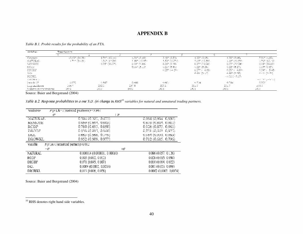
APPENDIX B

Table B.1. Probit results for the probability of an FTA.

Source: Baier and Bergstrand (2004)

ÝÞ ßàá âJã ä ã åáæ çèé æ á çê è ß Þ ßë à ëì ë áæ ì è Þ èé á íã îã ïð ñò óôõ ö÷ øõ ùú û10 variables for natural and unnatural trading partners.

Source: Baier and Bergstrand (2004)

10 RHS denotes right hand side variables.

41