arX

iv:p

hysi

cs/0

1120

56v1

[ph

ysic

s.ed

-ph]

19

Dec

200

1

physics/0112056

Linearisation of Simple Pendulum

P. Arun1 & Naveen Gaur2

Department of Physics & Astrophysics

University of Delhi

Delhi - 110 007, India

Abstract

The motion of a pendulum is described as Simple Harmonic Motion (SHM) in case

the initial displacement given is small. If we relax this condition then we observe the

deviation from the SHM. The equation of motion is non-linear and thus difficult to explain

to under-graduate students. This manuscript tries to simplify things.

1arunp92@yahoo.co.in2naveen@physics.du.ac.in, pgaur@ndf.vsnl.net.in

One of the basic experiments which a physics student will try out is that of the pendulum.

A pendulum consists of a massive bob suspended from a massless string, in actual terms, the

string does have a mass but it is negligible as compared to the mass of the bob. Also, for

making the assumption that the bob is a point mass, the length of the string is made far

greater than the radius of the bob.

The general equation of motion (EOM) of pendulum was derived in our previous work

[1, 2]. The equation [1] was :

cosΘ

2

d2Θ

dt2−

1

2sin

Θ

2(dΘ

dt)2 = − ω2 sinΘ (1)

In above eq.(1) Θ is the angular displacement and ω =√

g

l, where the terms have their usual

meaning. This is a non-linear differential equation and is not solvable analytically. We adopted

numerical methods to get the solutions of this equation under various conditions. If the initial

displacement is small, i.e. under small oscillation approximation we can write sinθ ∼ θ and

cosθ ∼ 1. Using this, eq.(1) goes to

d2Θ

dt2−

1

4Θ(

dΘ

dt)2 = − ω2Θ (2)

the second term on the left side of above eqn. is a second order term in Θ, so we can neglect

this term being the higher order term (in Θ) . So the eqn becomes

d2Θ

dt2= − ω2Θ (3)

this is the equation of SHM. So under small oscillation approximation the EOM of non-linear

pendulum turns to a linear second order differential equation in time, more well known as the

simple harmonic motion.

Let’s now discuss the solutions of both linear (eq.(3)) and non-linear (eq.(1)) equations.

As we discussed earlier work [2] that the eq.(1) can’t be solved analytically, so we tried out

numerical solution for the non-linear equation. But the solutions of linear equation(3) are well

known and can be written as :

Θi(t) = ACos(ωit) + BSin(ωit) (4)

2

where A and B are the constants (we expects two constants to be there in the general solution as

the equation which we are trying to solve is a second order equation in time), and ωi =√

2πTi

,

where the i subscript indicates that the EOM is SHM i.e. a linear second order equation.

The solution (equation 4) is a harmonic function of time. One can determine the unknown

coefficients A and B by using the initial conditions.

-1.5

-1

-0.5

0

0.5

1

1.5

2

0 0.2 0.4 0.6 0.8 1 1.2 1.4 1.6

displace

ment

a

t = 5 sect = 10 sect = 15 sect = 20 sec

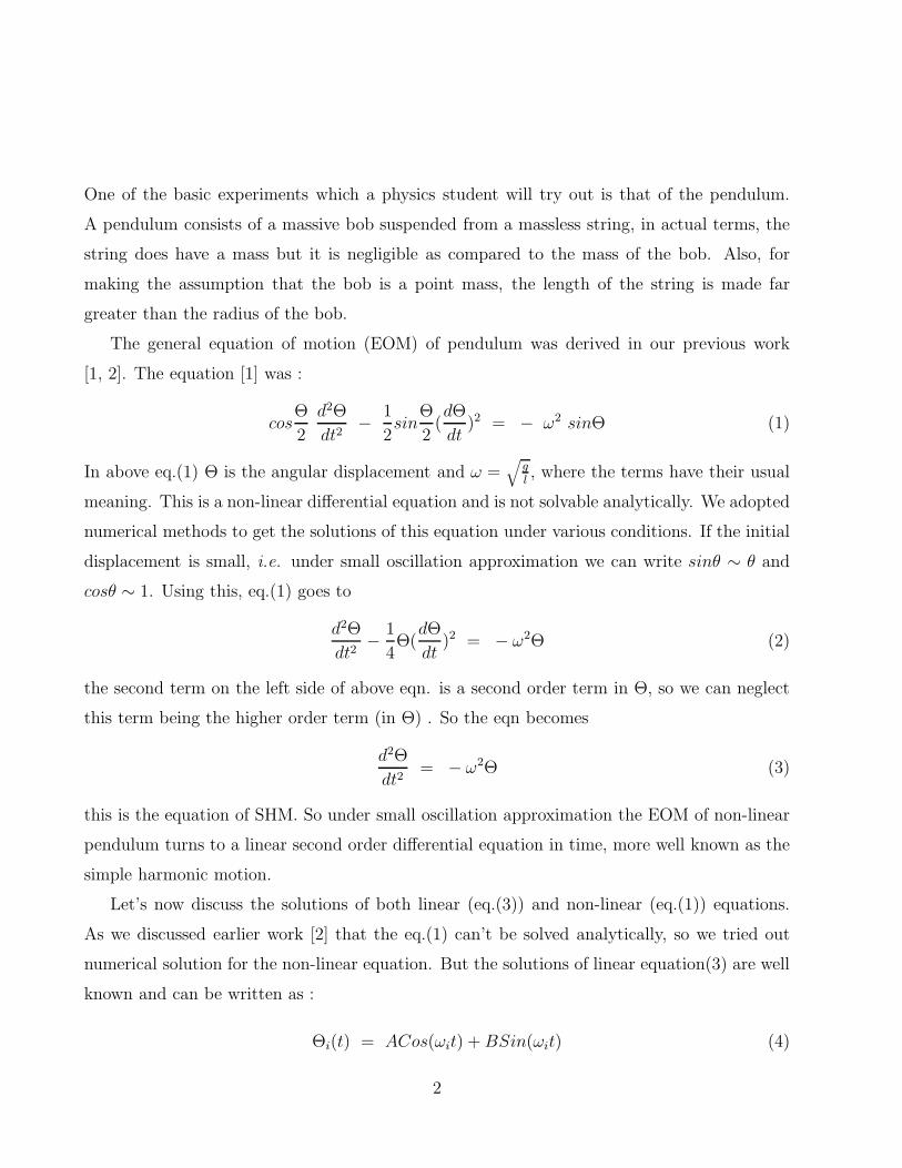
Figure 1: The plot of the displacement at various times (t = 5, 10, 15, 20 seconds) with the

initial displacement, ω = 4

For a simple pendulum the total time taken for completing N oscillations can be written

as :

t = T1 + T2 + . . . + TN (5)

where T1, T2, . . .TN are time periods of first, second, . . . and N th oscillation respectively. For

a simple pendulum undergoing SHM all the time periods are same i.e.

T1 = T2 = . . . = TN = Ti (6)

3

leading to

ti = NTi (7)

where the subscript i indicates the SHM. However in the case of pendulum obeying the non-

linear EOM (eq.(1), as we have shown in previous work [2], the time period of oscillation won’t

be the same as in the case of SHM (in fact the displacement given by non-linear EOM lags

behind in phase to that of SHM). Let’s parameterise this lag in phase by saying that a constant

phase difference (say α) is introduced to the time period after each successive oscillation i.e.

T = Ti − α (8)

where T is the time period of the pendulum using non-linear EOM. So after N oscillations the

difference between the two times would be

t = ti − Nα (9)

where t and ti are the time taken to complete N oscillations by the non-linear and linear oscil-

lators respectively, while α is the small variation introduced with each successive oscillations.

As time increases, the pendulum whose motion is described by eq(1) completes more oscilla-

tions as compared to the simple pendulum, for a given time. Thus, the only correction called

for seems to be a correction factor in the angular frequency. As we have also shown earlier

[2] that the difference between the two time periods increases as the initial amplitude of the

oscillation increases. So we can say that the correction factor is dependent of the initial dis-

placement. Also, for the initial displacement tending to be small, the correction factor should

approach zero and hence the non-linear oscillator should approach the SHM. So effectively we

can say that the motion of non-linear oscillator can still the thought of simple harmonic, with

the difference that the frequency is now dependent on the initial amplitude. So we can write

solution of actual pendulum of type :

Θ(t) = a Cos(ωit + f(a)t) (10)

where the constant A has been replaced with initial amplitude a. The function f(a) is the

function of initial displacement as argued above .

4

0

0.01

0.02

0.03

0.04

0.05

0.06

0.2 0.4 0.6 0.8 1 1.2 1.4 1.6

phase

diff

a

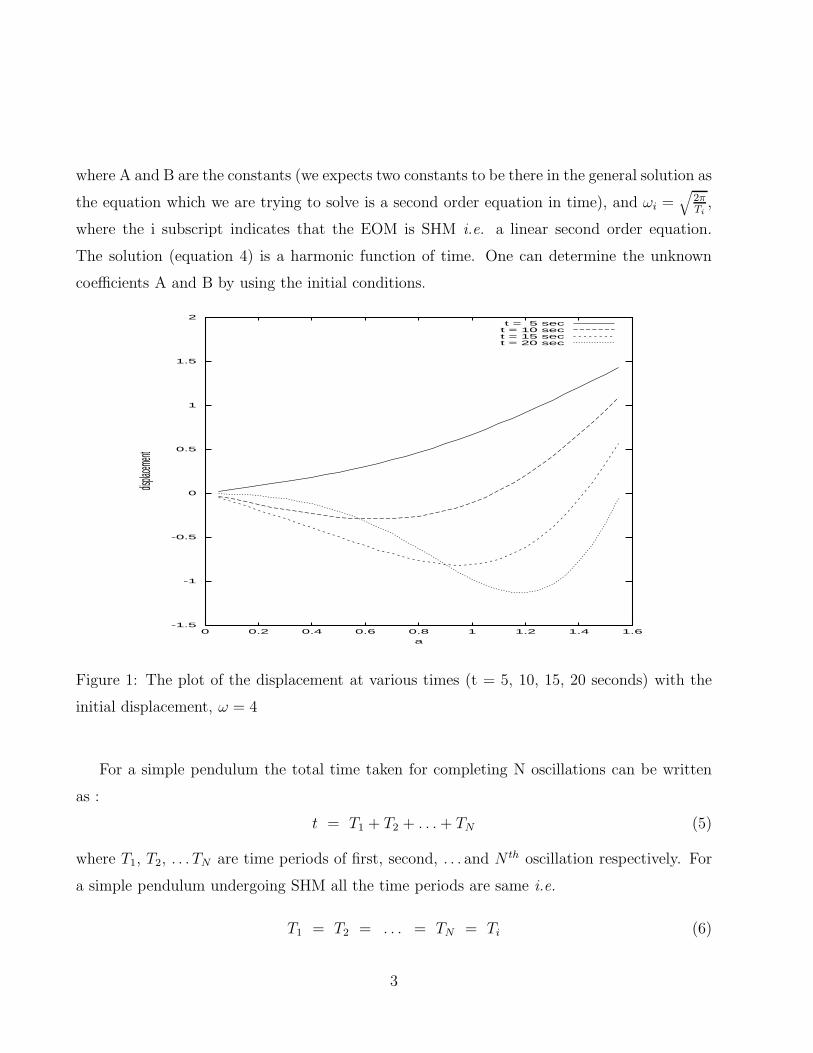
Figure 2: Plot of phase difference, between the solution of linear and nonlinear EOM of simple

pendulum, after the first oscillation. ω = 4

In figure () we have plotted the displacement at various times with the initial displacement.

In figure(2) we have plotted the phase difference introduced between the two displacements

which we get by solving the linear (SHM) eqn.(3) and the non-linear eq.(1) after the first

oscillation w.r.t. the initial displacement. As stated, α is the constant delay introduced in

successive oscillations, hence it is sufficient to plot between initial displacement and α after

the first oscillation. As can be seen f(α) is essentially a function of the initial displacement.

We have also tried to fit polynomial function of f(a) to the numerical results which we get by

solving eq.(1), the result is :

f(a) = a + bx + cx2 (11)

with

a = −0.0016674238 , b = 0.0026202282 , c = 0.024899586

5

Conclusion

In summary we have shown the difference in the results when we use the linear EOM (eq.(3) and

non-linear EOM (eq.(4) for describing a pendulum. The time taken to complete an oscillation

decreases with successive oscillations for a pendulum whose initial displacement is large. In

short it seems that under this condition the oscillator will oscillate more rapidly. Thus, in case

of a pendulum oscillating under the non-linear EOM condition, a modified value of ω has to

be considered which is a function of the initial displacement. Apart from this modification the

solution of non-linear EOM can also be taken to be harmonic.

References

[1] Peter V. O’Neil, “Advanced Engineering Mathematics”, 3ed edition, PWS publishing

company, Boston, 1993.

[2] P.Arun & Naveen Gaur, physics/0106097.

6