Embed Size (px)
Citation preview

Di r ecci ó n:Di r ecci ó n: Biblioteca Central Dr. Luis F. Leloir, Facultad de Ciencias Exactas y Naturales, Universidad de Buenos Aires. Intendente Güiraldes 2160 - C1428EGA - Tel. (++54 +11) 4789-9293
Co nta cto :Co nta cto : [email protected]
Tesis Doctoral
Medicion del flujo de neutrinosMedicion del flujo de neutrinoscósmicos ultra enérgeticos con elcósmicos ultra enérgeticos con el
detector de superficie deldetector de superficie delObservatorio Pierre AugerObservatorio Pierre Auger
Guardincerri, Yann
2013
Este documento forma parte de la colección de tesis doctorales y de maestría de la BibliotecaCentral Dr. Luis Federico Leloir, disponible en digital.bl.fcen.uba.ar. Su utilización debe seracompañada por la cita bibliográfica con reconocimiento de la fuente.
This document is part of the doctoral theses collection of the Central Library Dr. Luis FedericoLeloir, available in digital.bl.fcen.uba.ar. It should be used accompanied by the correspondingcitation acknowledging the source.
Cita tipo APA:
Guardincerri, Yann. (2013). Medicion del flujo de neutrinos cósmicos ultra enérgeticos con eldetector de superficie del Observatorio Pierre Auger. Facultad de Ciencias Exactas y Naturales.Universidad de Buenos Aires.
Cita tipo Chicago:
Guardincerri, Yann. "Medicion del flujo de neutrinos cósmicos ultra enérgeticos con el detectorde superficie del Observatorio Pierre Auger". Facultad de Ciencias Exactas y Naturales.Universidad de Buenos Aires. 2013.

UNIVERSIDAD DE BUENOS AIRESFacultad de Ciencias Exactas y Naturales
Departamento de Fısica
Medicion del flujo de neutrinos cosmicos ultraenergeticos con el detector de superficie del
Observatorio Pierre Auger
Trabajo de Tesis para optar por el tıtulo de
Doctor de la Universidad de Buenos Aires en el area Ciencias Fısicas
por Yann Guardincerri
Directores de Tesis: Prof. Ricardo Nestor Piegaia y Prof. Jaime Alvarez Muniz
Lugar de Trabajo: Dpto. Fısica - FCEyN - UBA
Buenos Aires, Argentina
24 de junio de 2013


Resumen
Medicion del flujo de neutrinos cosmicos ultra energeticos con eldetector de superficie del Observatorio Pierre Auger
El Detector de Superficie del Observatorio Pierre Auger es sensible a tau neutrinos
que cruzan la Tierra de forma rasante interactuando en su corteza. Los leptones tau
que surgen de las interacciones via corriente cargada pueden emerger de la Tierra
y decaer en la atmosfera produciendo lluvias de partıculas casi horizontales que
contienen una componente electromagnetica significativa. En esta tesis se disenan
tecnicas de reconstruccion y de identificacion que permiten distinguir estas lluvias
de las producidas por rayos cosmicos iniciados por protones o nucleos de hierro,
usando como observable la estructura temporal de las senales que se detectan en los
detectores de agua que miden radiacion de Cherenkov. Se describe el procedimiento
de busqueda de neutrinos, el metodo desarrollado para calcular la exposicion del ob-
servatorio y las incertezas sistematicas asociadas. Ningun candidato a neutrino fue
encontrado en los datos adquiridos entre 1 de Enero del 2004 hasta 31 de Diciembre
del 2012. Asumiendo un flujo diferencial Φ(Eν) = k ·E−2ν , se fija un lımite superior
con un nivel de confianza del 90% al flujo difuso de neutrinos de todos los sabores de
k < 5× 10⁻⁸ GeV cm−2 s−1 sr−1 en el intervalo de energıas de 1017 eV a 1019.1 eV.
Se testean modelos astrofısicos concretos de produccion de neutrinos, y se derivan
lımites a flujos de fuentes puntuales en funcion de su declinacion.
Palabras claves: astropartıculas, neutrinos cosmogenicos , neutrinos UHE, rayos
cosmicos, Observatorio Pierre Auger
iii

iv
Abstract
Measurement of the ultra-high energy cosmic neutrino flux with theSurface Detector array at the Pierre Auger Observatory
The Surface Detector of the Pierre Auger Observatory is sensitive to Earth-skimming
tau neutrinos that interact in Earth’s crust. Tau leptons from charged-current in-
teractions can emerge and decay in the atmosphere to produce a nearly horizontal
shower with a significant electromagnetic component. In this thesis techniques are
developed to reconstruct and distinguish these showers from the ones produced by
regular hadronic cosmic rays by the broad time structure of the signals in the water-
Cherenkov detectors. The neutrino search procedure, the method to compute the
observatory exposure and the associated systematic uncertainties are described. No
neutrino candidate has been found in data collected from 1 January 2004 to 31
December 2012. Assuming a differential flux Φ(Eν) = k · E−2ν in the energy range
from 1017 eV− 1019.1 eV, we place a 90% CL upper limit on the all flavour neutrino
diffuse flux of k < 5 × 10⁻⁸ GeV cm−2 s−1 sr−1. Concrete astrophysical neutrino
models are tested and limits to point-like source fluxes are derived as a function of
declination.
Keywords: astroparticles, cosmogenic neutrinos, UHE neutrinos, cosmic rays,
Pierre Auger Observatory
v

vi

Acknowledgments
Mi experiencia en el Observatorio Pierre Auger fue excelente. Voy a estar siem-
pre agradecido a mis directores Ricardo Piegaia y Jaime Alvarez Muniz. Fue un
inmenso placer trabajar bajo su tutela y aprender de ellos en diferentes aspectos de
mi formacion. Los dos me dejaron un ejemplo gigante de lo que significa trabajar
en ciencia.
Estoy profundamente agradecido con Javier Tiffenberg. Para mi sos un grande!
No tengo palabras para agradecerte todo lo que me ensenaste y ayudaste durante
estos anos.
Hay mucha gente de la colaboracion que contribuyo mediante discusiones con mi
trabajo de doctorado. Particularmente quiero agradecerle a Enrique Zas, Gonzalo
Parente, Sergio Navas, Jose Luis Navarro, Mathieu Tartare, Pierre Billoir, Markus
Roth, Carla Bonifazi, Isabelle Lhenry-Yvon, Piera Ghia, Paolo Privitera, Diego
Harari y Esteba Roulet.
Estoy infinitamente agradecido a mi familia. A mis papas, Carlos e Ines, quienes
me formaron como persona y lo siguen haciendo cada dıa con su ejemplo. Muchısimas
gracias por ser como son, por su incondicional amor y apoyo durante todos estos
anos de esfuerzo para que pueda alcanzar mis objetivos. A mi hermano que me
muestra lo que significa la pasion y la lealtad. Gracias Lu! Te admiro montones.
A mis primos, tıos y abuelos, quienes siempre estan cuando necesito una mano. En
especial a Gusti, Caro y Sampipit que me prestaron la oreja cuando necesitaba hacer
catarsis.
A mis amigos gracias por estar durante todos estos anos de esfuerzo, por compar-
tir asados, noches de teg y mucho mas. En especial a Santi quien sabe mostrarme
mis falencias.
A toda la gente del grupo experimental de altas energıas del Departamento:
Hernan, Pablo, Laura, Gaston, Sabrina, Orel y Gustavo. En particular, gracias
Pablo por ser mi companero de aventuras en Auger durante los ultimos anos, gracias
Hernan por cada vez que te pedı ayuda y encontraste el tiempo para tratar de
responder y gracias Gustavo por tus consejos.
Hay mucha mas gente que estuvo muy presente durante mi paso por la Facultad.
vii

viii
En particular, muchas gracias a Mati, Diego, Tifi, Fede, Guille y tantos mas.
Me gustarıa resaltar mi agradecimiento a toda la gente que trabaja para que la
Facultad de Ciencias Exactas y Naturales funcione. Esta Institucion tiene mucho
que ver en mi formacion como persona y me siento extremadamente orgulloso de
haber pertenecido a ella durante los ultimos anos.
Por ultimo, pero de importancia mayuscula quiero agradecerle a Tef, el cuore
de mi cuore, por la paciencia de estos ultimos meses y por compartir los suenos de
futuro. Me diste la fuerza para terminar!
Contents
1 Introduction 1
1.1 Why ultra-high energy neutrinos? . . . . . . . . . . . . . . . . . . . . 2
1.2 Potential Sources of Diffuse Neutrino Flux . . . . . . . . . . . . . . . 4
1.2.1 GZK Neutrinos . . . . . . . . . . . . . . . . . . . . . . . . . . 5
1.2.2 Active Galactic Nuclei and Gamma Ray Bursts . . . . . . . . 8
1.2.3 Unconventional Neutrino Sources . . . . . . . . . . . . . . . . 10
1.2.4 Theoretical limits on Neutrino Flux . . . . . . . . . . . . . . . 11
1.3 Experimental searches . . . . . . . . . . . . . . . . . . . . . . . . . . 12
1.3.1 Optical Methods . . . . . . . . . . . . . . . . . . . . . . . . . 13
1.3.2 Radio Cherenkov . . . . . . . . . . . . . . . . . . . . . . . . . 13
1.3.3 Cosmic Ray Detectors . . . . . . . . . . . . . . . . . . . . . . 16
2 Neutrino detection using atmospheric showers 19
2.1 Atmospheric particle showers . . . . . . . . . . . . . . . . . . . . . . 19
2.1.1 Model of the evolution of EAS . . . . . . . . . . . . . . . . . . 21
2.1.2 Heitler model: electromagnetic shower . . . . . . . . . . . . . 22
2.1.3 Showers produced by protons or nuclei . . . . . . . . . . . . . 23
2.1.4 Inclined showers . . . . . . . . . . . . . . . . . . . . . . . . . . 24
2.2 Neutrino showers . . . . . . . . . . . . . . . . . . . . . . . . . . . . . 25
2.2.1 Atmospheric neutrino induced showers . . . . . . . . . . . . . 25
2.2.2 Earth-skimming tau neutrino induced showers . . . . . . . . . 27
2.3 Detection techniques . . . . . . . . . . . . . . . . . . . . . . . . . . . 28
2.3.1 Surface detector methods . . . . . . . . . . . . . . . . . . . . . 28
3 The Pierre Auger Observatory 31
3.1 Surface Detector . . . . . . . . . . . . . . . . . . . . . . . . . . . . . 31
3.1.1 Surface detector calibration . . . . . . . . . . . . . . . . . . . 33
3.1.2 Trigger system and data aqcuisition . . . . . . . . . . . . . . . 36
ix

x Contents
4 Monte Carlo simulations: neutrinos 41
4.1 Earth processes . . . . . . . . . . . . . . . . . . . . . . . . . . . . . . 41
4.1.1 Neutrino Interaction . . . . . . . . . . . . . . . . . . . . . . . 42
4.1.2 Tau Propagation . . . . . . . . . . . . . . . . . . . . . . . . . 44
4.1.3 Monte Carlo simulations . . . . . . . . . . . . . . . . . . . . . 48
4.2 Atmospheric simulation . . . . . . . . . . . . . . . . . . . . . . . . . . 51
4.2.1 Simulation of τ decay . . . . . . . . . . . . . . . . . . . . . . 52
4.2.2 Atmospheric shower . . . . . . . . . . . . . . . . . . . . . . . 54
4.2.3 Surface detector response . . . . . . . . . . . . . . . . . . . . . 56
4.3 Weights . . . . . . . . . . . . . . . . . . . . . . . . . . . . . . . . . . 57
5 Reconstruction and selection of inclined showers 61
5.1 Selection of quality events . . . . . . . . . . . . . . . . . . . . . . . . 61
5.1.1 Photomultiplier tube selection . . . . . . . . . . . . . . . . . . 62
5.1.2 Station selection . . . . . . . . . . . . . . . . . . . . . . . . . 65
5.1.3 Preliminary reconstruction with accidental station removal . . 70
5.1.4 Additional selection . . . . . . . . . . . . . . . . . . . . . . . . 72
5.2 Variables for selection of inclined showers . . . . . . . . . . . . . . . . 73
5.2.1 Event footprint . . . . . . . . . . . . . . . . . . . . . . . . . . 73
5.2.2 Ground speed . . . . . . . . . . . . . . . . . . . . . . . . . . . 74
5.3 Performance of the inclined shower selection . . . . . . . . . . . . . . 74
5.3.1 Events with 4 stations or more . . . . . . . . . . . . . . . . . 75
5.3.2 Events with 3 stations . . . . . . . . . . . . . . . . . . . . . . 75
5.4 Summary . . . . . . . . . . . . . . . . . . . . . . . . . . . . . . . . . 81
6 Neutrino identification 83
6.1 Subdivision of the data sample . . . . . . . . . . . . . . . . . . . . . . 84
6.2 Selection: Idea and potential variables . . . . . . . . . . . . . . . . . 86
6.3 Selection of young showers: previous analysis . . . . . . . . . . . . . . 89
6.4 New Selection Strategy . . . . . . . . . . . . . . . . . . . . . . . . . . 91
6.5 Neutrino event selection and background estimation . . . . . . . . . . 96
6.5.1 Events with 3 stations . . . . . . . . . . . . . . . . . . . . . . 99
6.6 Training and Test data samples comparison . . . . . . . . . . . . . . 101
6.6.1 Time evolution of the mean 〈AoP〉 distribution . . . . . . . . 102
6.6.2 Compatibility of the tails of the distributions in the Training
and Test samples . . . . . . . . . . . . . . . . . . . . . . . . . 103
6.6.3 Remarks and Conclusions . . . . . . . . . . . . . . . . . . . . 104
6.7 Summary . . . . . . . . . . . . . . . . . . . . . . . . . . . . . . . . . 105
Contents xi
7 Detector efficiency and exposure 107
7.1 Detector efficiency . . . . . . . . . . . . . . . . . . . . . . . . . . . . 107
7.1.1 Infinite detector efficiency . . . . . . . . . . . . . . . . . . . . 107
7.1.2 Finite detector efficiency . . . . . . . . . . . . . . . . . . . . . 111
7.2 Exposure . . . . . . . . . . . . . . . . . . . . . . . . . . . . . . . . . . 113
7.2.1 Exposure definition . . . . . . . . . . . . . . . . . . . . . . . . 113
7.2.2 Temporal evolution of the SD . . . . . . . . . . . . . . . . . . 114
7.2.3 Exposure calculation . . . . . . . . . . . . . . . . . . . . . . . 116
7.2.4 Exposure results . . . . . . . . . . . . . . . . . . . . . . . . . 121
7.2.5 Systematic Uncertainties . . . . . . . . . . . . . . . . . . . . . 123
8 Results and discussion 129
8.1 Blind search: “opening the box” . . . . . . . . . . . . . . . . . . . . . 129
8.2 Comparison to theory: statistical treatment . . . . . . . . . . . . . . 131
8.3 Testing theoretical predictions . . . . . . . . . . . . . . . . . . . . . . 134
8.4 Upper limit on the diffuse flux . . . . . . . . . . . . . . . . . . . . . . 136
8.4.1 Integral limit . . . . . . . . . . . . . . . . . . . . . . . . . . . 137
8.4.2 Quasi-differential limit . . . . . . . . . . . . . . . . . . . . . . 139
8.5 Point Sources . . . . . . . . . . . . . . . . . . . . . . . . . . . . . . . 140
9 Conclusions 145


1Introduction
The field of astroparticle physics is currently undergoing rapid development. The
traditional messenger on the sky, the photon, has been complemented starting early
last century by charged cosmic rays observations and, during the last decades, by
the development of neutrino astrophysics. They are all rich messengers allowing us
to probe the properties of astrophysical sources.
Neutrino astronomy is only just beginning. It has the possibility to open a new
window on the universe, expanding what is possible to know about astrophysical
phenomena. Charged cosmic rays are deflected by magnetic fields and gamma rays
can be absorbed by intervening material or pair produce on photon backgrounds
prevalent throughout the universe. Neutrinos suffer from neither problem since
they are neutral and only interact via the weak force. Even though they are difficult
to observe particle astrophysicists are stepping up to the challenge. The era of ded-
icated high-energy neutrino telescopes began in earnest a couple of decades ago and
it promises to open a new and exciting window on the Universe. There are several
extensive reviews [1] highlighting the potential physics and astrophysics objectives
using the neutrino messenger.
In this dissertation, we focus on the search of neutrinos in the energy interval
between 1017 eV to 1020 eV with the Pierre Auger Observatory. This thesis is or-
ganized as follows. In this Chapter we review the present status of theoretical and
experimental neutrino astrophysics. Chapter 2 describes extended air showers and,
in particular, the ones produced by neutrinos. Chapter 3 presents an overview of
the Pierre Auger Observatory. The processes involved in neutrino simulations are
explained in Chapter 4. The reconstruction and identification of neutrinos is the
subject of Chapters 5 and 6. In Chapter 7 we detail the determination of the obser-
vatory exposure, i.e., its sensitivity to cosmological neutrinos. Chapter 8, finally, is
dedicated to the search results and the comparison with theoretical predictions.
1
2 1.1 Why ultra-high energy neutrinos?
1.1 Why ultra-high energy neutrinos?
The study of charged ultra-high energy cosmic rays (UHECRs) has stimulated
much experimental and theoretical activity in the field of Astroparticle Physics. Al-
though, their energy spectrum is measured over an astonishing energy range covering
14 orders of magnitude, many mysteries remain to be solved, such as their origin
and production mechanism. In particular, charged UHECRs measurements suffer
from two limitations, source pointing and the GZK cutoff.
At energies below 1019.5 eV, charged particles trajectories are substantially bent
by galactic and intergalactic magnetic fields and their arrival direction on Earth
does not point back to their source of origin.
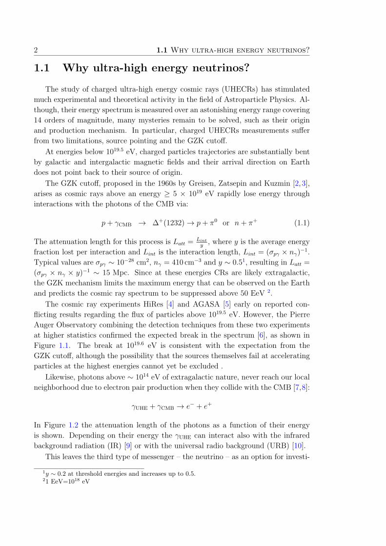
The GZK cutoff, proposed in the 1960s by Greisen, Zatsepin and Kuzmin [2, 3],
arises as cosmic rays above an energy ≥ 5 × 10¹⁹ eV rapidly lose energy through
interactions with the photons of the CMB via:
p+ γCMB → ∆+(1232) → p+ π0 or n+ π+ (1.1)
The attenuation length for this process is Latt =Lint
y, where y is the average energy
fraction lost per interaction and Lint is the interaction length, Lint = (σpγ × nγ)−1.
Typical values are σpγ ∼ 10−28 cm2, nγ = 410 cm−3 and y ∼ 0.51, resulting in Latt =
(σpγ × nγ × y)−1 ∼ 15 Mpc. Since at these energies CRs are likely extragalactic,
the GZK mechanism limits the maximum energy that can be observed on the Earth
and predicts the cosmic ray spectrum to be suppressed above 50 EeV 2.
The cosmic ray experiments HiRes [4] and AGASA [5] early on reported con-
flicting results regarding the flux of particles above 1019.5 eV. However, the Pierre
Auger Observatory combining the detection techniques from these two experiments
at higher statistics confirmed the expected break in the spectrum [6], as shown in
Figure 1.1. The break at 1019.6 eV is consistent with the expectation from the
GZK cutoff, although the possibility that the sources themselves fail at accelerating
particles at the highest energies cannot yet be excluded .
Likewise, photons above ∼ 1014 eV of extragalactic nature, never reach our local
neighborhood due to electron pair production when they collide with the CMB [7,8]:
γUHE + γCMB → e− + e+
In Figure 1.2 the attenuation length of the photons as a function of their energy
is shown. Depending on their energy the γUHE can interact also with the infrared
background radiation (IR) [9] or with the universal radio background (URB) [10].
This leaves the third type of messenger – the neutrino – as an option for investi-
1y ∼ 0.2 at threshold energies and increases up to 0.5.21 EeV=1018 eV

1 Introduction 3
Figure 1.1 The UHECR spectrum obtained by the Pierre Auger Observatory. Itis fitted with three power-law functions (dashed) and two power-law plus a smoothfunction (solid line). Only statistical uncertainties are shown. The systematic un-certainty on the energy scale is 22%.
-2
-1
0
1
2
3
4
5
12 14 16 18 20 22
CMB
URBIR
red shift limit
Log(L/
Mpc
)
Log(E/eV)
γ
Figure 1.2 Attenuation length L for photons [11]. Photons with energy between1014 and 1018 eV cannot reach the Earth if created at distances larger than 1 Mpc.Labels IR, CMB and URB (see text) indicate the dominant background againstwhich the γUHE interact.
4 1.2 Potential Sources of Diffuse Neutrino Flux
gation at the highest reaches of astrophysics. Indeed, soon after the GZK mechanism
was proposed, it was realized that high energy neutrinos, which we call cosmogenic
or GZK neutrinos, were a natural by-product of that process through its consequent
pion decay [12, 13]:
π+ → µ+ + νµ → e+ + νe + νµ + νµ (1.2)
Neutrinos do not suffer from any of the aforementioned disadvantages. They
interact only through the weak interaction with a very small cross section. They
travel cosmological distances without interacting and, moreover, if they are produced
at the source, they escape from the object without loosing energy. As they are
electrically neutral, they will not be bent by the magnetic fields of the universe and
point back to their origin. Therefore, neutrinos are unique messengers with which we
can probe the possible sources of cosmic rays and study the mechanism of UHECR
interaction during their propagation in the Universe. Furthermore, with energies
above 1017 eV, they would produce interactions with nucleons at center-of-mass
energies near 100 TeV, exceeding those achieved at terrestrial accelerators. This
provides a laboratory to search for new physics beyond the scope of the Standard
Model of particle physics.
In the following sections of this chapter, we will present a discussion of astrophys-
ical neutrino sources and fluxes, namely from the GZK mechanism, Active Galactic
Nuclei (AGNs) and Gamma Ray Bursts (GRBs). We also briefly survey past, cur-
rent and future experimental endeavors in the field.
1.2 Potential Sources of Diffuse Neutrino Flux
Various models in the literature predict UHE neutrinos and estimate their co-
rresponding fluxes. As mentioned, the observations of CRs above 50 EeV and a
cutoff in the spectrum imply the likely existence of cosmogenic neutrinos. In this
case the neutrinos are produced during the propagation of UHECRs through the
Universe. They could also potentially be produced by the acceleration of protons
and nuclei in active galactic nuclei (AGN) [14], or by photopion production in cos-
mological gamma ray burst (GRB) [15]. Detectors such as AMANDA, or IceCube,
its successor, are well-suited to search for sources with strong power-law (∼ E−2 )
energy spectra that extends from TeV to above the PeV scales. Sources that emit
neutrinos with energy spectra that peak at energies above 100 PeV are expected to
have lower fluxes which require detectors with larger exposures.
It has been previously speculated that UHE neutrinos could also possibly be
associated with the decays of extremely massive exotic particles such as topological
defects [16], or the interaction of energetic neutrinos with Big-Bang relic cosmic
background neutrinos via the Z-burst resonance [17]. These ideas, primarily moti-
1 Introduction 5
vated to explain the highest energies cosmic rays, have now been severely constrained
by recent experiments. A review can be be found in [18]. In the next subsections
we summarize the main ideas.
1.2.1 GZK Neutrinos
Greisen, Zatsepin and Kusmin proposed that as cosmic rays with energies greater
than 5 × 10¹⁹ eV propagate in the universe, they interact with the cosmic microwave
background and generate neutrinos via pion decay, equation1.2.
The presence of the GZK cutoff hint that UHECRs are likely to be extragalactic.
This implies that GZK neutrinos are the most secure predictions for neutrino fluxes
in the energy interval between 1016 eV and 1021 eV. Nevertheless there are significant
theoretical uncertainties in the calculations as we see next.
Estimates of the flux and shape of the GZK neutrino flux depend on the following
factors [19–23]:
1. Composition of UHECRs,
2. UHECR energy spectrum (spectral shape, normalization and energy cutoff),
3. Cosmological model,
4. Cosmological evolution of the sources with redshift,
5. Proton-photon cross section, and
6. Neutrino oscillations.
1. Composition of UHECR
The first predictions of the cosmogenic neutrino flux assumed that the UHECR
primaries were pure protons. More recent cosmogenic neutrino fluxes calculations
[20, 24] take pure 56Fe, 4He, or 16O and mixtures of these nuclei with protons as
the primaries. The heavier nuclei lose energy via photo-disintegration, in which
secondary nucleons are produced. The photopion production of these secondary
nucleons creates UHE neutrinos. In addition, a small flux of anti-electron neutrinos
are produced via neutron decays [25] but the energies are too small to be of interest
to Auger. For non-pure proton composition, the neutrino flux is small compared
with that expected from a pure proton component [24]. The energy per nucleon
after photo-disintegration is much smaller than the primary energy (in the case of
Fe, EA
∼ Ep
56) and may be too low to interact by the GZK process. Some neutrino
flux estimations assume the sources inject a mixture of primaries with the same
initial abundances as the observed Galactic cosmic rays [22]. Changing the primary
component produces an uncertainty in the prediction of neutrino fluxes of more than
an order of magnitude.
6 1.2 Potential Sources of Diffuse Neutrino Flux
Recent experimental results by Auger [26] , though highly debated, indicate that
the flux of UHECRs may be dominated by heavier nuclei. This is at variance with
the results from HiRes, and more recently, Telescope Array (TA) [27]. Conversely,
if neutrino fluxes are observed above the predictions from a large Z cosmic ray com-
position, they will shed light on the elemental composition of extragalactic cosmic
ray sources or even rule out heavy composition.
2. Energy profile
The injection spectrum of UHECR can be inferred from experimental results of
cosmic ray detectors on Earth. Typically it is assumed that the UHECR spectrum
at injection is a power-law with the following energy dependence:
dN
dE= P0 × E−α × exp (− E
Ec
) (1.3)
where P0 is a normalization constant. The spectral index α lies between 1.8 and 2.7,
favored to be close to α ≈ 2.3. The cutoff energy at injection, Ec , is assumed to be
between 1020 eV and 1023 eV. The values of α and Ec are both dependent on the
corresponding source characteristics and the acceleration mechanism of cosmic rays
at the source. Once the spectral index and cutoff energy are set, the normalization
is chosen so that the propagated CRs at Earth fit the observed CR spectrum. A
steeper injection spectrum and smaller cutoff energy generate smaller neutrino fluxes
at 1018 - 1019 eV due to the decreased number of protons at high energies that would
be responsible for such neutrinos.
3. Cosmological model
The cosmology of the Universe is another factor that drives the uncertainty of
the GZK neutrino flux. Astrophysical observations now point to models with a
cosmological constant Λ [28], compared with the flat, mass dominated Einstein-de
Sitter Universe (ΩM = 1) typically assumed by calculations prior to mid-90’s. The
currently favored model is one with ΩΛ = 0.7 and ΩM = 0.3 [29], which means
that dark energy accounts for 70% of the total mass-energy of the Universe. Con-
sequently, the Universe was expanding less quickly during the epoch that generated
cosmological ν’s leading to a proportionally larger contribution to the neutrino yield
from higher redshifts. Engel et al. [19] compared the neutrino fluxes derived from the
two cosmological models and found that the ΩΛ = 0.7 model increases the neutrino
flux by 60% for a moderate redshift evolution.
4. Cosmological evolution
Predictions of neutrino fluxes are strongly dependent on the cosmological evolu-
tion of the potential cosmic ray sources. There are at least four evolution models
that have been most commonly discussed in the literature, namely:
i. No evolution,
ii. Star Formation Rate (SFR),

1 Introduction 7
iii. Active Galactic Nuclei-FRII (FRII) and
iv. Strong Gamma Ray Burst (GRB).
When describing the cosmological evolution of sources, a source evolution term
H(z) is used to specify evolution of mass (or rate) density of sources with redshift
z within a comoving volume. It represents the ratio of the mass density of sources
between redshift z and now. The mass density of sources at redshift of z would be
ρ(z) = H(z)× ρ(0).
i. No evolution: The simplest model assumes that there is no evolution with
redshift (i.e. H(z) = 1) and it yields the most conservative neutrino flux.
ii. SFR: This model was first introduced in [30] and then studied in more detail
in [31]. They use data from different experiments measuring the number of sources
as a function of redshift to infer when were the stars formed. In this model, the
density of sources first increases, then remains constant or with a small decrease
and, finally, there is a cutoff. As an example we show the parametrization given
in [31]:
H(z) ∝
(1 + z)3.4 z < 1,
(1 + z)−0.3 1 < z < 4.5
(1 + z)−8 z > 4.5
iii. FRII: Radio galaxies are a kind of active galaxy very luminous at radio
wavelengths. One way of classifying these galaxies is by the morphology of the
large-scale radio emission. FRI galaxies typically have bright jets in the centre,
while FRIIs have faint jets but bright hotspots at the ends of the lobes. FRI are far
from satisfying the energetic criteria to accelerate particles to the highest energies
[32]. FRIIs appear to be able to transport energy efficiently to the ends of the
lobes, although it is worth mentioning that no outstanding correlation has been
observed between catalogues of FRII galaxies and the most energetic events seen
by the Pierre Auger Collaboration. The distribution of these sources as a function
of redshift is described in [33]. In order to compare with SFR we present here a
simple approximation to the distribution: increasing faster than in the case of SFR
((1 + z)4) until redshifts of 2 and then decreasing as exp [(2− z)/1.5] 3. The effect
of this kind of source evolution on the expected neutrino flux is studied in [22] and
the result is an enhancement of the flux in a factor 7 with respect to the SFR.
iv. GRB: The latest Swift observations indicate that the GRB rate departs
from the SFR rate at the highest redshifts (z > 4) [34]. However, the difference
in the expected neutrino fluxes between SFR and GRB is very small because the
contribution of sources at redshifts z > 4 is less than 1% to the total flux due to the
redshift dilution.3The parametrization used in [22] is 2.7z + 1.45z2 + 0.18z3 − 0.01z4.
8 1.2 Potential Sources of Diffuse Neutrino Flux
5. Proton-photon cross-section
The neutrino yield from the interaction:
pγ → ∆+ → n+ π+ → n+ νµ + e+ + νe + νµ (1.4)
is determined by the proton-photon cross-section, σpγ. Cross-section measurements
from accelerator data are used to estimate the fraction of energy going into neutrinos
and the number of neutrinos produced in one interaction. Generally, it is assumed
that the fraction of energy going into the charged pion from the proton is on average
xp→π ≈ 0.2 and that the four leptons carry an equal amount of energy, so on average
each neutrino carries about 1/20 of the proton energy. The energy carried by a
neutrino in a neutron decay is only ∼ 3 × 10⁻⁴ times the energy of the origina
proton [35].
6. Neutrino oscillations
In the decay of a pion the ratio of muon neutrinos to electron neutrinos is about
2. In this work, unless stated otherwise, muon neutrinos (νµ) refer to νµ + νµ, and
the same applies for electron neutrinos (νe) and tau neutrinos (ντ ). Due to the fact
than neutrino oscillate, original cosmic neutrino fluxes with a νe : νµ : ντ ratio at
the source of 1:2:0 oscillate to a ratio of 1:1:1.
Though the existence of cosmogenic neutrinos is very likely, flux predictions span
four orders of magnitude. Some of these predictions are shown in Fig. 1.3 for the
total neutrino flux summed over all three flavors.
1.2.2 Active Galactic Nuclei and Gamma Ray Bursts
Active Galactic Nuclei (AGN) are the most persistent objects isotropically dis-
tributed in the sky and one of the most powerful source classes with luminosities
on the order of 1045±3 erg/s [36]. Therefore they are considered as one of the best
candidate sources for UHE cosmic ray production and many authors predict mea-
surable fluxes of neutrinos if the acceleration site is surrounded by a sufficiently
thick cocoon of material.
The enormous radiation from AGNs is thought to be fueled by gravitational
energy released as matter infalls onto a supermassive black hole at its center. During
this process, angular momentum causes the material to flatten into an accretion
disk. Infalling matter is diverted into a perpendicular oriented jet, with turbulent
shocks accelerating particles to high energies. Thereby, a significant fraction of
gravitational energy is converted into highly relativistic particles via first-order Fermi
acceleration [37] of charged particles. Frictional heating turns the infalling matter
into plasma, which thereby produces a strong magnetic field. The collisions of
ultra-relativistic protons with the intense photon fields of AGN yield high energy
1 Introduction 9
[eV]νE1710 1810 1910 2010 2110
]-1
sr
-1 s
-2)
[
GeV
cm
ν(E
Φ ν2k
= E
-1110
-1010
-910
-810
-710
-610
-510Cosmogenic neutrino fluxes (all flavour)
[eV]νE1710 1810 1910 2010 2110
]-1
sr
-1 s
-2)
[
GeV
cm
ν(E
Φ ν2k
= E
-1110
-1010
-910
-810
-710
-610
-510Engel et al
Yuksel et al
Ahlers et al, Fermi-LAT bound
Allard et alsee details in textevolution: FRIIcomposition: iron
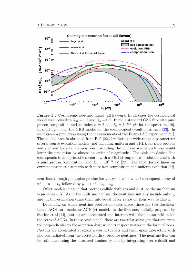
Figure 1.3 Cosmogenic neutrino fluxes (all flavour): In all cases the cosmologicalmodel used considers ΩM = 0.3 and ΩΛ = 0.7. In red a standard GZK flux with pureproton composition and an index α = 2 and Ec = 1021.5 eV for the spectrum [19].In solid light blue the GRB model for the cosmological evoultion is used [23]. Insolid green a prediction using the measurements of the Fermi-LAT experiment [21].The shaded area is obtained from Ref. [22], bracketing a wide range a parameters:several source evolution models (not including uniform and FRII), for pure protonsand a mixed Galactic composition. Including the uniform source evolution wouldlower the prediction by almost an order of magnitude. The pink dot-dashed linecorresponds to an optimistic scenario with a FRII strong source evolution case witha pure proton composition, and Ec = 1021.5 eV [22]. The blue dashed lineis anextreme pessimistic scenario with pure iron composition and uniform evolution [22].
neutrinos through photopion production via pγ → π+ + n and subsequent decay of
π+ → µ+ + νµ followed by µ+ → e+ + νe + νµ.
Other models imagine that protons collide with gas and dust, so the mechanism
is pp → πs +X. As in the GZK mechanism, the neutrinos initially include only νµand νe, but oscillation turns them into equal flavor ratios on their way to Earth.
Depending on where neutrino production takes place, there are two classifica-
tions: AGN core model or AGN jet model. In the first one, initially proposed by
Stecker et al [14], protons are accelerated and interact with the photon field inside
the cores of AGNs. In the second model, there are two relativistic jets that are emit-
ted perpendicular to the accretion disk, which transport matter in the form of lobes.
Protons are accelerated at shock waves in the jets and then, upon interacting with
photons radiated from the accretion disk, produce neutrinos. The neutrino flux can
be estimated using the measured luminosity and by integrating over redshift and
10 1.2 Potential Sources of Diffuse Neutrino Flux
luminosity [38]. Mannheim et al. [39] calculated the maximum possible neutrino
flux originating from AGNs using source evolution functions for blazars and varying
the energy where the cosmic ray spectrum changes its slope.
Gamma Ray Bursts (GRBs) are brief flashes of γ-ray emitted by sources at
cosmological distances. They are the most energetic explosions in the Universe and
are thought to be possible sources of high energy neutrinos. Their neutrino emissions
have been calculated under various scenarios.
In the currently favored GRB fireball shock model [42,43], the prompt γ rays are
produced by collisions of plasma material moving relativistically along a jet (internal
shocks), i.e. a fireball. Late time collisions of jetted material with an external
medium, like interstellar medium (external shocks), produce a broad band radiation
like X-ray, UV and optical radiation, collectively known as the GRB afterglow.
In the jet, electrons and protons are accelerated by relativistic shocks via Fermi
mechanism. The synchrotron radiation and inverse Compton scattering by the high
energy electrons lead to the observed prompt photons. The accelerated protons
on the other hand interact with observed prompt γ-rays or afterglow photons via
photopion production interaction, and produce a burst of high energy neutrinos
accompanying the GRB. The neutrinos generated in the original fireball with internal
shock are called burst neutrinos, and those from GRB external shock are called
afterglow neutrinos.
Another popular GRB model is the supernova model [44] in which a supernova
remnant shell from the progenitor star is ejected prior to the GRB burst. Protons
in the supernova remnant shell and photons entrapped from a supernova explosion
or a pulsar wind from a fast-rotating neutron star remnant provide ample targets
for protons accelerated in the internal shocks of the gamma-ray burst to interact
and produce high energy neutrinos.
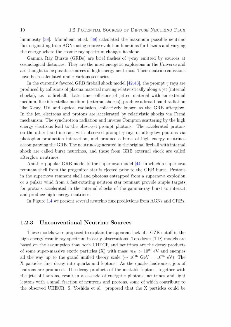
In Figure 1.4 we present several neutrino flux predictions from AGNs and GRBs.
1.2.3 Unconventional Neutrino Sources
These models were proposed to explain the apparent lack of a GZK cutoff in the
high energy cosmic ray spectrum in early observations. Top-down (TD) models are
based on the assumption that both UHECR and neutrinos are the decay products
of some super-massive exotic particles (X) with mass mX > 1020 eV and energies
all the way up to the grand unified theory scale (∼ 1016 GeV = 1025 eV). The
X particles first decay into quarks and leptons. As the quarks hadronize, jets of
hadrons are produced. The decay products of the unstable leptons, together with
the jets of hadrons, result in a cascade of energetic photons, neutrinos and light
leptons with a small fraction of neutrons and protons, some of which contribute to
the observed UHECR. S. Yoshida et al. proposed that the X particles could be
1 Introduction 11
[eV]νE1710 1810 1910 2010 2110
]-1
sr
-1 s
-2)
[
GeV
cm
ν(E
Φ ν2k
= E
-1110
-1010
-910
-810
-710
-610
-510AGN and GRB neutrino fluxes (all flavour)
[eV]νE1710 1810 1910 2010 2110
]-1
sr
-1 s
-2)
[
GeV
cm
ν(E
Φ ν2k
= E
-1110
-1010
-910
-810
-710
-610
-510AGN
MPR-max
BBR
Stecker
GRB
WB
RMW-afterglow
Figure 1.4 Predicted neutrino fluxes from AGNs and GRBs(all flavour): In blackwe show three different models for AGNs [39–41] and in red two models for GRBs[43,44].
released from topological defects, such as monopoles and cosmic strings, which were
formed in the early universe; and that the UHECR well above 1020 eV and UHE
neutrinos are the result of the annihilation or collapse of topological defects [16].
The Z-Burst model proposed that neutrinos may not only be cosmological by-
products but could also be the sources of UHECR. This model was presented when
AGASA reported a flux of particles above 1019 eV which was not suppresed by the
GZK cutoff. It assumes a large flux of neutrinos at energies of order 1022−23 eV.
These can annihilate with Big-Bang relic cosmic background neutrinos (Tν ∼ 1.9 K)
in our own Galactic halo via the interaction as: ν + ν → Z0 [17]. The decays of the
neutral weak vector boson Z0 yields UHECRs, while the high energy neutrinos that
do not interact could be detected at the Earth.
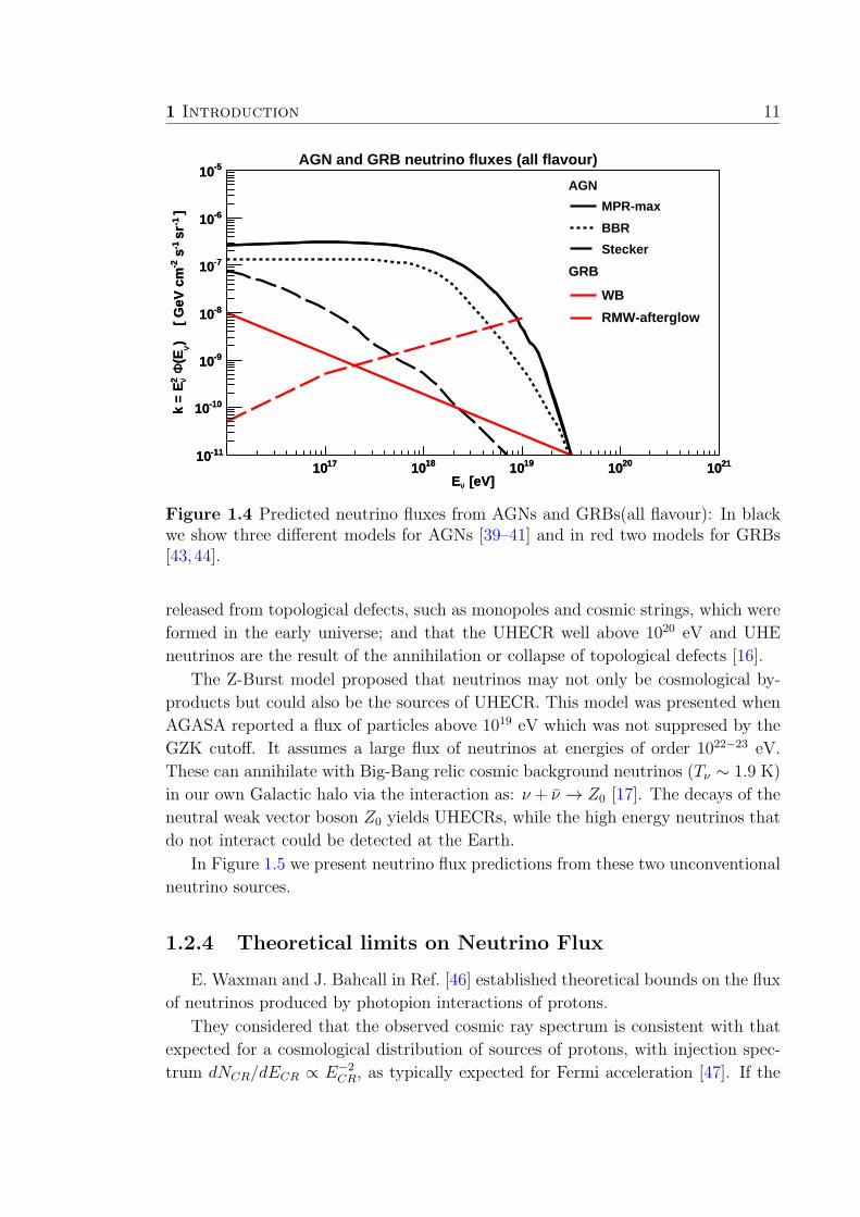
In Figure 1.5 we present neutrino flux predictions from these two unconventional
neutrino sources.
1.2.4 Theoretical limits on Neutrino Flux
E. Waxman and J. Bahcall in Ref. [46] established theoretical bounds on the flux
of neutrinos produced by photopion interactions of protons.
They considered that the observed cosmic ray spectrum is consistent with that
expected for a cosmological distribution of sources of protons, with injection spec-
trum dNCR/dECR ∝ E−2CR, as typically expected for Fermi acceleration [47]. If the
12 1.3 Experimental searches
[eV]νE1710 1810 1910 2010 2110
]-1
sr
-1 s
-2)
[
GeV
cm
ν(E
Φ ν2k
= E
-1110
-1010
-910
-810
-710
-610
-510Unconventional neutrino fluxes (all flavour)
[eV]νE1710 1810 1910 2010 2110
]-1
sr
-1 s
-2)
[
GeV
cm
ν(E
Φ ν2k
= E
-1110
-1010
-910
-810
-710
-610
-510TD
Z-Burst
Figure 1.5 Neutrino fluxes from unconventional sources (all flavour): A modelconsidering a super-massive (mX ≥ 2× 10²³ eV) exotic particle decay and a Z-burstmodel [45].
high-energy protons produced by the extra-galactic sources lose a fraction ǫ < 1 of
their energy through photo-meson production of pions before escaping the source,
for energy independent ǫ the resulting present-day energy density of muon neutrinos
follows the proton generation spectrum. Assuming that all the energy injected as
high-energy protons is converted to pions via photopion or p-p collision, the energy
generation rate of neutrinos cannot exceed the energy generation rate of protons
at the sources. Using this energy-dependent generation rate of cosmic-rays they
derived a characteristic E−2 spectrum bound on the muon neutrino flux (νµ and νµcombined) for the cosmological model of no redshift evolution and for a Quasi Stellar
Objects cosmological model. To get an upper bound on the total neutrino flux, the
muon neutrino intensities are multiplied by 1.5 due to the ratio of νe : νµ : ντ= 1 :
2 : 0 at the origin.
It is important to emphasize that the calculations produce an upper bound.
There are no lower bounds in the literature.
1.3 Experimental searches
We review4 some current and upcoming experiments that are involved in searches
for UHE neutrinos of cosmic origin. The detection techniques rely on Cherenkov
radiation, either in optical or radio for the very highest energies. Acoustic detectors
4Many extensive reviews and status reports appear in the literature. Ref [48] provide concisesummary of astrophysical neutrino searches.
1 Introduction 13
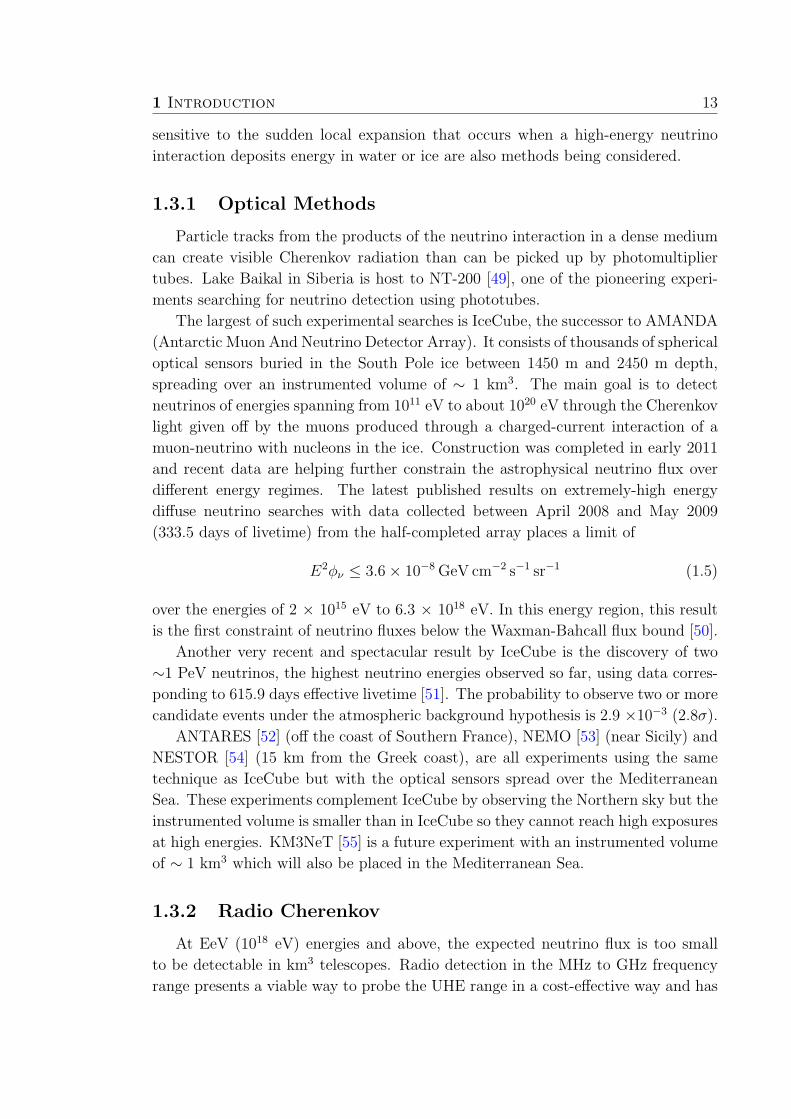
sensitive to the sudden local expansion that occurs when a high-energy neutrino
interaction deposits energy in water or ice are also methods being considered.
1.3.1 Optical Methods
Particle tracks from the products of the neutrino interaction in a dense medium
can create visible Cherenkov radiation than can be picked up by photomultiplier
tubes. Lake Baikal in Siberia is host to NT-200 [49], one of the pioneering experi-
ments searching for neutrino detection using phototubes.
The largest of such experimental searches is IceCube, the successor to AMANDA
(Antarctic Muon And Neutrino Detector Array). It consists of thousands of spherical
optical sensors buried in the South Pole ice between 1450 m and 2450 m depth,
spreading over an instrumented volume of ∼ 1 km3. The main goal is to detect
neutrinos of energies spanning from 1011 eV to about 1020 eV through the Cherenkov
light given off by the muons produced through a charged-current interaction of a
muon-neutrino with nucleons in the ice. Construction was completed in early 2011
and recent data are helping further constrain the astrophysical neutrino flux over
different energy regimes. The latest published results on extremely-high energy
diffuse neutrino searches with data collected between April 2008 and May 2009
(333.5 days of livetime) from the half-completed array places a limit of
E2φν ≤ 3.6× 10⁻⁸ GeV cm−2 s−1 sr−1 (1.5)
over the energies of 2 × 10¹⁵ eV to 6.3 × 10¹⁸ eV. In this energy region, this result
is the first constraint of neutrino fluxes below the Waxman-Bahcall flux bound [50].
Another very recent and spectacular result by IceCube is the discovery of two
∼1 PeV neutrinos, the highest neutrino energies observed so far, using data corres-
ponding to 615.9 days effective livetime [51]. The probability to observe two or more
candidate events under the atmospheric background hypothesis is 2.9 ×10⁻³ (2.8σ).
ANTARES [52] (off the coast of Southern France), NEMO [53] (near Sicily) and
NESTOR [54] (15 km from the Greek coast), are all experiments using the same
technique as IceCube but with the optical sensors spread over the Mediterranean
Sea. These experiments complement IceCube by observing the Northern sky but the
instrumented volume is smaller than in IceCube so they cannot reach high exposures
at high energies. KM3NeT [55] is a future experiment with an instrumented volume
of ∼ 1 km3 which will also be placed in the Mediterranean Sea.
1.3.2 Radio Cherenkov
At EeV (1018 eV) energies and above, the expected neutrino flux is too small
to be detectable in km3 telescopes. Radio detection in the MHz to GHz frequency
range presents a viable way to probe the UHE range in a cost-effective way and has

14 1.3 Experimental searches
been proposed as an avenue for neutrino detection by Gurgen Askaryan in the early
1960’s [57] [56]. He realized that the coherence of the Cherenkov radiation in the
radio regime results in the power of the pulse being proportional to the square of the
primary of energy of the initial particle. Coupled with the fact that the attenuation
lengths in naturally occurring media like ice, salt and sand is very long (hundreds
of meters) at such frequencies (1 GHz), it is promising to instrument large volume
of such media to listen to RF pulses. All the past, present and proposed radio
Cherenkov experiments use one of these three media.
RICE (the Radio Ice Cherenkov Experiment) searches for radio emission from
electromagnetic and hadronic cascades induced by UHE neutrinos colliding with
nuclei in the Antarctic ice. It is an array of 16 antennas of bandwidth 200-1000
MHz contained within a cube of ice 200 m on a side, with a center about 150 m
deep, near the South Pole. Based on data collected from 1999 to 2005, with a
livetime of 74.1 × 10⁶ s, RICE placed a 95% CL model-dependent limits on the
neutrino flux of all flavors of
E2φν ≤ 10−6 GeV cm−2 s−1 sr−1 (1.6)
over the energy regime of 1017 eV to 1020 eV [57], after no neutrino candidate events
were found. For similar comparison with other flux limits, we scale the limit to 90%
C.L. in Figure 1.6.
ANITA (ANtarctic Impulsive Transient Array) is an Antarctic balloon-borne
experiment that is launched under NASA’s balloon program from the McMurdo
station. It consists of an array of broadband (200-1200 MHz) dual-polarization
quadridged horn antennas that observes the Antarctic ice sheet from its in-flight
altitude of 37 km. The first full ANITA flight, following the ANITA-LITE prototype
test flight in early 2004, was launched on December 2006 and remained aloft above
Antartica for 35 days [58].
The second flight, with a payload enhanced from 32 to 40 antennas and other
hardware improvement, was in December 2008. From 28.5 days livetime and using
one observed candidates, ANITA-II set a 90% CL integral flux limit on all neutrino
flavors of
E2φν ≤ 1.3× 10⁻⁷ GeV cm−2 s−1 sr−1 (1.7)
the strongest constraint to date over the energy range 1018 eV to 1023.5 eV [59].
GLUE (Goldstone Lunar Ultrahigh Energy) searched for ∼10 ns microwave
pulses from the lunar soil, appearing in coincidence at two large radio telescopes
separated by about 20 km and linked by optical fiber. The pulses can arise from
subsurface electromagnetic cascades induced by interactions of up-going UHE neu-
trinos in the lunar regolith. Using data of about 30 hours of livetime which yielded
zero events, GLUE sets upper limits on the diffuse cosmic neutrino fluxes over the
energy range from 1019 eV to 1022.5 eV [60]. Kalyazin [61] and Parkes [62] experi-

1 Introduction 15
ments have also previously monitored the moon for signals. There are ongoing efforts
to exploit either existing radio telescopes like Westerbork Synthesis Radio Telescope
through the NuMoon [63], and future giant arrays like the planned Square Kilometer
Array (SKA), that is to be located in South Africa or Australia [64]. LUNASKA
(Lunar UHE Neutrino Astrophysics using the Square Kilometer Array) is one such
proposal, with first preparatory observations taken with the ATCA (Australian Tele-
scope Compact Array) [65].
ARA (Askaryan Radio Array) is an initiative to develop a multi-phased teraton-
scale ultra- high energy neutrino detector in deep, radio-transparent ice near the
South Pole [66]. A station design consists of a cluster of 16 embedded antennas
deployed up to 200 m deep in several vertical boreholes placed with tens-of-meter
horizontal spacing to form a small sub-array. An initial prototype detector system
was installed in January 2011 to perform studies relating to the radio environment
of the site: background noise levels and radio clarity of the ice. There are plans to
build a 200 km2 array, known as ARA-37.
ARIANNA (Antarctic Ross Ice-shelf ANtenna Neutrino Array) [67] aims at
using the enormous Ross Ice Shelf near the coast of Antarctica. It is designed to
detect UHE neutrinos with energy greater than 1017.5 eV. The concept emerged
following recent studies [68] at the Ross Ice Shelf that confirmed earlier glaciological
surveys that found high fidelity radio reflectivity of the ice-water bottom. This
would allow for detection of the reflected conical Cherenkov pulses generated by
“down-going” neutrinos arriving from the whole southern celestial hemisphere . The
advantages are low levels of anthropogenic radio noise in Antarctica, the possibility
of long livetime and the scalability to large volumes attainable by covering vast
expanses of the area with autonomous radio antenna stations.
SalSA (Salt Sensor Array) is a detector concept to deploy radio detectors in
one of the large salt formations (a few km2 × 10 km are not atypical) that exist in
many locations around the world [69]. One would find 2.5 times as many neutrino
interactions per unit volume in salt compared to ice due to its higher density. Al-
though the peak power of the emitted radio Cherenkov signal is lower than in ice,
the width of the Cherenkov cone is broader [70]. Additionally, an experiment in
the Northern Hemisphere would observe a region of the sky not in the field of view
of an experiment in the South. Ground Penetrating Radar (GPR) experts have re-
ported low radio loss in salt mines in the US, but it is difficult to deduce attenuation
lengths measurements from their findings [71]. Before a SalSA experiment can move
forward, long attenuation lengths (250 m) must be measured definitively at radio
frequencies.

16 1.3 Experimental searches
1.3.3 Cosmic Ray Detectors
We have already introduced three cosmic ray experiments that were involved in
the determination of the GZK cutoff. Though designed for UHECR studies, they
can be used to observe neutrinos.
AGASA (Akeno Giant Air Shower Array) used a widely spread ground array,
consisting of 111 plastic scintillation detectors of 2.2 m2 over an area of 100 km2
with a separation of 1 km, to detect UHECR by measuring the secondary particles
produced in a cosmic ray shower [5].
The HiRes (High Resolution Fly’s Eye) experiment consists of two detector
stations located 12.6 km apart. Each station monitors its surrounding sky for ob-
serving fluorescent emission from cosmic ray air showers in atmosphere [4]. The
GZK feature in their measurements has been corroborated by Auger, as seen earlier
in Figure 1.1. However, they diverge on other CR observations: no anisotropy in
their smaller data sample and light primaries composition persistent up to the higher
energies. Regarding neutrino detection, they have reported 90% C.L integrated flux
limits E2φν of 3.81 × 10⁻⁷ , 9.73 × 10⁻⁷ and 4.71 × 10⁶ GeV cm−2 sr−1 s−1 over
three decades energy centered around 1018.5 , 1019.5 and 1020.5 respectively. This
calculation was based on a livetime of 3638 hours, with no neutrino events, and
combining results from ντ and νe studies [72]. They were sensitive to decays of the
outgoing tau’s following ντ interactions in the Earth’s crust and to electromagnetic
showers induced by the νe also interacting in the Earth’s crust [73].
Auger (Pierre Auger Observatory) hybrids both techniques of surface and fluo-
rescence detectors to observe showers simultaneously [74]. It can detect UHE neu-
trinos by searching for extended inclined air shower from down-going neutrinos of
any flavor or up-going tau neutrinos through a distinctive broad signal in time as
their signature. In the first case, the neutrino can interact at any atmospheric depth
to produce an extensive air shower [75]. Earth skimming UHE ντ s may undergo a
charged-current interaction to produce τs close to the surface, which can exit the
Earth and decay in the atmosphere to produce a nearly horizontal electromagnetic
shower [76]. Based on the published data taken until May 2010, an upper limit on
the diffuse flux of UHE ντ is set at 90% C.L. for Earth-skimming neutrinos,
E2φν ≤ 9.6× 10⁻⁸ GeV cm−2 s−1 sr−1 (1.8)
in the energy range 2 × 10¹⁷ eV < Eν < 2 × 10¹⁹ eV [77], and for downward-going
neutrinos,
E2φν ≤ 5.1× 10⁻⁷ GeV cm−2 s−1 sr−1 (1.9)
in the energy range 1 × 10¹⁷ eV < Eν < 1 × 10¹⁹ eV [75]. For better comparison
with other experiments, we have converted from single flavour to all flavours limits
by multiplying by 3.

1 Introduction 17
In Figure 1.6, we summarize the flux limits imposed in the 1017 -1021 eV energy
range.
[eV]νE1710 1810 1910 2010 2110
]-1
sr
-1 s
-2)
[
GeV
cm
ν(E
Φ ν2k
= E
-1110
-1010
-910
-810
-710
-610
-510Experimental upper limits to neutrino fluxes (all flavour) 90% CL
[eV]νE1710 1810 1910 2010 2110
]-1
sr
-1 s
-2)
[
GeV
cm
ν(E
Φ ν2k
= E
-1110
-1010
-910
-810
-710
-610
-510
Auger Earth-skimming (Jan 04 - May 10)
Auger downward-going (Nov 07 - May 10)
RICE (4.8 yr)
IceCube-40 (333.5 days)
ANITA-II (28.5 days)
Figure 1.6 Limits for a diffuse neutrino flux of all flavors from the Pierre AugerObservatory [75, 77], RICE [57] (scaled to 90% C.L.), IceCube (IC-40) [50] andANITA-2 [59]. The IceCube energy range of the integral limit is 2 × 10¹⁵ eV to 6.3× 10¹⁸ eV. The ANITA-2 energy range of the integral limit is 1018 eV to 1023.5 eV.

2Neutrino detection usingatmospheric showers
The principle of detection of neutrinos using extended atmospheric showers, EAS,
is the subject of this Chapter. Section 2.1 introduces the phenomenon of EAS
discussing the differences between vertical and inclined showers. In Section 2.2
we describe the characteristics of showers initiated by neutrinos interacting in the
atmosphere and in the Earth crust. In Section 2.3 the detection technique to measure
these showers is explained.
2.1 Atmospheric particle showers
At the end of the 30’s Pierre Auger observed that the trigger coincidence be-
tween cosmic ray detectors which were separated by several kilometers was higher
than expected for independent events. He proposed an explanation postulating the
existence of very energetic particles which generated new particles when they in-
teracted high in the atmosphere. The first generation of new particles could again
interact and produce a further generation, initiating a chain reaction which mul-
tiplied the number of particles. The phenomenon is known today as an extended
atmopheric shower, EAS.
After 70 years of research, the structure and evolution of particle showers is
considered to be well understood. After the first interaction, the development can
be described as a set of particles of high energy (usually hadrons), which travel along
the axis of the shower producing less energetic electrons, muons and photons that
diffuse over the radial direction (see Fig. 2.1). In this way, the EAS are a thin disk
of particles which propagates close to the speed of light in a path determined by
the direction of the primary particle. This disk, also called front, presents a high
19
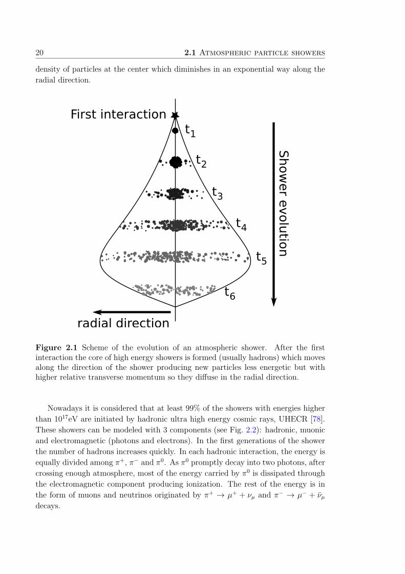
20 2.1 Atmospheric particle showers
density of particles at the center which diminishes in an exponential way along the
radial direction.
Shower evolution
radial direction
t1
t5
t4
t3
t2
t6
First interaction
Figure 2.1 Scheme of the evolution of an atmospheric shower. After the firstinteraction the core of high energy showers is formed (usually hadrons) which movesalong the direction of the shower producing new particles less energetic but withhigher relative transverse momentum so they diffuse in the radial direction.
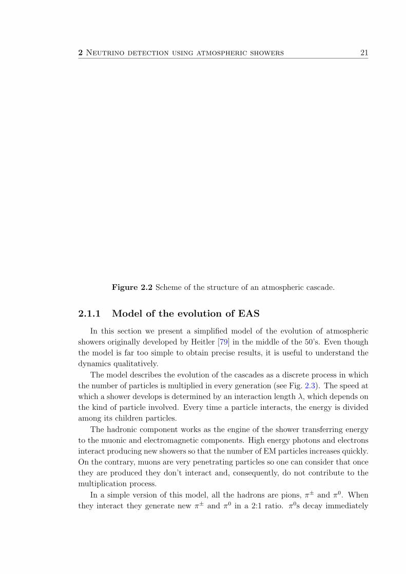
Nowadays it is considered that at least 99% of the showers with energies higher
than 1017eV are initiated by hadronic ultra high energy cosmic rays, UHECR [78].
These showers can be modeled with 3 components (see Fig. 2.2): hadronic, muonic
and electromagnetic (photons and electrons). In the first generations of the shower
the number of hadrons increases quickly. In each hadronic interaction, the energy is
equally divided among π+, π− and π0. As π0 promptly decay into two photons, after
crossing enough atmosphere, most of the energy carried by π0 is dissipated through
the electromagnetic component producing ionization. The rest of the energy is in
the form of muons and neutrinos originated by π+ → µ+ + νµ and π− → µ− + νµdecays.
2 Neutrino detection using atmospheric showers 21
Primary cosmic ray
π+
π-
π0
γe+
e-
Electromagnetic
component
Muonic
component
Hadronic
component
atmospheric nuclei
ν
μ+μ-
Top of the atmosphere
Figure 2.2 Scheme of the structure of an atmospheric cascade.
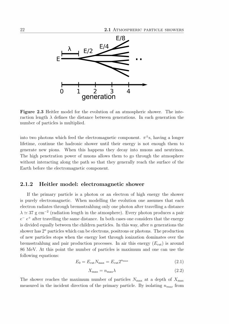
2.1.1 Model of the evolution of EAS
In this section we present a simplified model of the evolution of atmospheric
showers originally developed by Heitler [79] in the middle of the 50’s. Even though
the model is far too simple to obtain precise results, it is useful to understand the
dynamics qualitatively.
The model describes the evolution of the cascades as a discrete process in which
the number of particles is multiplied in every generation (see Fig. 2.3). The speed at
which a shower develops is determined by an interaction length λ, which depends on
the kind of particle involved. Every time a particle interacts, the energy is divided
among its children particles.
The hadronic component works as the engine of the shower transferring energy
to the muonic and electromagnetic components. High energy photons and electrons
interact producing new showers so that the number of EM particles increases quickly.
On the contrary, muons are very penetrating particles so one can consider that once
they are produced they don’t interact and, consequently, do not contribute to the
multiplication process.
In a simple version of this model, all the hadrons are pions, π± and π0. When
they interact they generate new π± and π0 in a 2:1 ratio. π0s decay immediately
22 2.1 Atmospheric particle showers
generation
Figure 2.3 Heitler model for the evolution of an atmospheric shower. The inte-raction length λ defines the distance between generations. In each generation thenumber of particles is multiplied.
into two photons which feed the electromagnetic component. π±s, having a longer
lifetime, continue the hadronic shower until their energy is not enough them to
generate new pions. When this happens they decay into muons and neutrinos.
The high penetration power of muons allows them to go through the atmosphere
without interacting along the path so that they generally reach the surface of the
Earth before the electromagnetic component.
2.1.2 Heitler model: electromagnetic shower
If the primary particle is a photon or an electron of high energy the shower
is purely electromagnetic. When modelling the evolution one assumes that each
electron radiates through bremsstrahlung only one photon after travelling a distance
λ ≃ 37 g cm−2 (radiation length in the atmosphere). Every photon produces a pair
e− e+ after travelling the same distance. In both cases one considers that the energy
is divided equally between the children particles. In this way, after n generations the
shower has 2n particles which can be electrons, positrons or photons. The production
of new particles stops when the energy lost through ionization dominates over the
bremsstrahlung and pair production processes. In air this energy (Ecut) is around
86 MeV. At this point the number of particles is maximum and one can use the
following equations:
E0 = EcutNmax = Ecut2nmax (2.1)
Xmax = nmaxλ (2.2)
The shower reaches the maximum number of particles Nmax at a depth of Xmax
measured in the incident direction of the primary particle. By isolating nmax from

2 Neutrino detection using atmospheric showers 23
equation 2.1 and introducing it in equation 2.2 one obtains the following expresion
for Xmax:
Xmax = λ log2
(E0
Ecut
)
(2.3)
Even though this model is very simple, this equation is capable of providing a rough
estimate of the depth Xmax. As an example, a 1018 eV photon reaches the maximum
quantity of particles at a depth of ∼ 800 g cm−2 [80], and the model predicts ∼1200
g cm−2.
2.1.3 Showers produced by protons or nuclei
In a shower initiated by a hadron, typically 80% of the particles produced in the
first interaction are pions (the rest being kaons, other mesons and nuclei-antinuclei
pairs). Secondary hadrons with enough energy continue the hadronic shower which
develops along the shower axis. Low energy mesons decay transferring their energy
to the EM and muonic components.
Neutral pions π0 have a lifetime of 8.4× 10⁻¹⁷s so they decay within a short dis-
tance1. The π0 decays electromagnetically2, producing electromagnetic sub-showers
identical to the ones described in Sec. 2.1.2. The size of the shower increases until
the energy of the electrons drops below the critical energy. At this point of the
shower, around 90% of the total energy is in the form of electrons and photons.
At lower energies, the losses through inoization overcome bremsstrahlung and the
electromagnetic component starts to diminish.
Electrons and positrons suffer multiple scattering which determines the charac-
teristics of the transversal structure of the shower.
Charged mesons have a larger lifetime (2.6× 10⁻⁸s), so they have a larger prob-
ability of interacting with atmopheric nuclei before decaying. The competition be-
tween the two processes depends essentially on the balance between the mean free
path of the interaction, which depends on the cross-section and the medium density,
and the decay length. Both of them vary with the energy and become the same at
∼ 115GeV for charged pions and ∼ 850GeV for kaons [80].
When kaons and pions decay they produce muons and νµ. The cross-section of
the interaction of neutrinos is negligible and they escape carrying around ∼2% of
the primary energy [80]. As the shower evolves, the muonic component increases
until reaching a maximum and then decreases very slowly because the decay length
is large3. Also muons loose energy at a much slower rate than electrons4.
Showers induced by hadrons have a spatial structure very different from the
1The decay length of a GeV (PeV) π0 is ∼0.2µm (0.2m).2The most frequent channel is into 2 photons (BR = 98.8%).3The decay length of a GeV (PeV) µ is ∼6km (6×10⁶km).4In air dE
dx(GeV (PeV)µ) ∼ 4(1000)MeVg−1cm2.
24 2.1 Atmospheric particle showers
ones initiated by electrons or photons. The latter are more compact due to the
fact that the transversal moment pT of electrons and photons is usually small. On
the contrary, deep inelastic scattering (DIS), typical in hadronic showers, usually
produces particles with high pT. Another important difference is that the hadronic
showers present a muonic component 100 times more abundant than the observed
in an EM shower. The few muons in an EM shower are the result of the decay of
pions produced in photonuclear reactions.
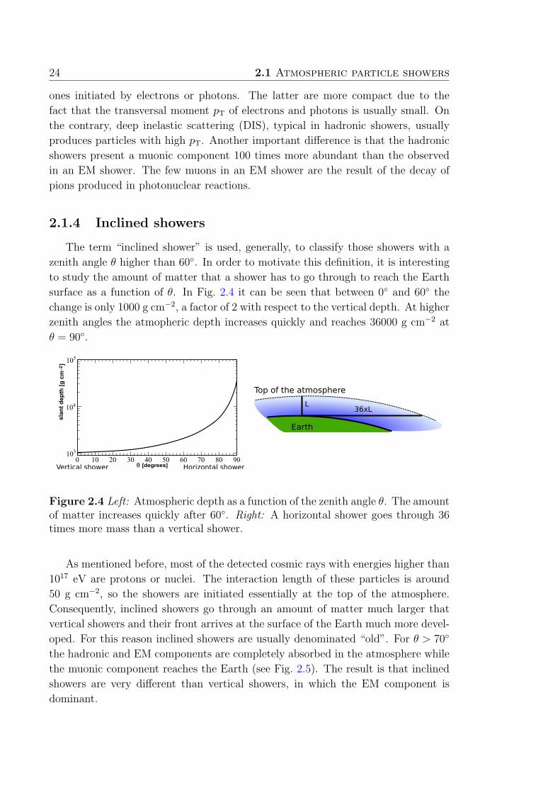
2.1.4 Inclined showers
The term “inclined shower” is used, generally, to classify those showers with a
zenith angle θ higher than 60. In order to motivate this definition, it is interesting
to study the amount of matter that a shower has to go through to reach the Earth
surface as a function of θ. In Fig. 2.4 it can be seen that between 0 and 60 the
change is only 1000 g cm−2, a factor of 2 with respect to the vertical depth. At higher
zenith angles the atmopheric depth increases quickly and reaches 36000 g cm−2 at
θ = 90.
Vertical shower Horizontal shower[degrees]
Earth
Top of the atmosphereL 36xL
Figure 2.4 Left: Atmospheric depth as a function of the zenith angle θ. The amountof matter increases quickly after 60. Right: A horizontal shower goes through 36times more mass than a vertical shower.
As mentioned before, most of the detected cosmic rays with energies higher than
1017 eV are protons or nuclei. The interaction length of these particles is around
50 g cm−2, so the showers are initiated essentially at the top of the atmosphere.
Consequently, inclined showers go through an amount of matter much larger that
vertical showers and their front arrives at the surface of the Earth much more devel-
oped. For this reason inclined showers are usually denominated “old”. For θ > 70
the hadronic and EM components are completely absorbed in the atmosphere while
the muonic component reaches the Earth (see Fig. 2.5). The result is that inclined
showers are very different than vertical showers, in which the EM component is
dominant.

2 Neutrino detection using atmospheric showers 25
hadronic
component
EM component
μ
proton or nucleiTop of the atmosphere
Earth
Figure 2.5 Inclined showers produced by protons or nuclei high in the atmosphere.The hadronic and EM components are absorbed and only muons reach the Earth.
2.2 Neutrino showers
2.2.1 Atmospheric neutrino induced showers
Within the Standard Model (SM), the neutrinos interact through the weak force.
They also interact through gravity, but in practice, only weak interactions allow to
detect individual neutrinos. The primary interaction of the neutrino is DIS. Fig. 2.6
summarizes the weak interaction channels. In all cases around 20% of the energy
of the primary neutrino is transferred to the hadronic jet which results from the
nucleon debris. These particles initiate cascades very similar to those produced by
protons. The remaining 80% of the energy of the primary particle is contained in a
ultra-energetic lepton. The actual energy that is transferred to the shower depends
on the interaction channel and neutrino flavour.
If the shower is initiated by a νe through charged current (CC), the resulting
electron initiates an electromagnetic shower overlapping the hadronic one produced
by the jet. In this case 100% of the energy is transferred to the shower. On the
contrary, neutral current interactions (NC) produce a secondary neutrino instead
of an electron. This neutrino escapes and does not contribute to the process of
multiplication, carrying around 20% of the energy of the primary neutrino.
Inclined showers initiated by a νµ through CC are very similar to the ones initi-
ated via NC even though the fundamental interaction is very different. At 1018 eV,
the probability that the high energy secondary muon decays before reaching the
surface is less than 10−6 and it decreases for higher energies 5. At the same time,
the probability of interacting and transferring an important amount of its energy
5The Earth radious R is ∼ 6000 km and the decay length λD of a EeV µ is ∼ 6 × 10⁹ km sothe probability is P = 1− exp (R/λD) = 1− exp (10−6) ∼ 10−6.

26 2.2 Neutrino showers
Neutral CurrentCharged Current
νx
νxHadronic
jet
νe
Hadronic
jet
High energy
electron
ντ
Hadronic
jet
νμ
μHadronic
jet
High energy
tauHigh energy
muon
nucleon hadronic jet
W
νe e
nucleon hadronic jet
W
νμ μ
nucleon hadronic jet
W
ντ τ
τ
nucleon hadronic jet
Z
νx νx
High energy
neutrino
Figure 2.6 Neutrino interaction channels according to the Standard Model. Inevery case the Feynman diagram is shown at the lowest order. In all channels theemerging jet of the broken nuclei initiate a hadronic shower. The electron producedin the interaction of a νe through CC generates also an electromagnetic shower whichis added to the hadronic. One ντ interacting through CC generates a high energy τthat can travel a distance which depends on its energy and produces a shower closerto the ground.
through bremsstrahlung or DIS is of the order of 10−3 [81]. Consequently, it is
indistinguishable from a secondary neutrino that emerges from a NC interaction.
The ντ via CC presents an interesting characteristic. In the same way as the
muon, the τ lepton is a very penetrating particle which can travel an important
distance from the point at which it was produced. On the other hand, its lifetime is
seven orders of magnitud lower so it can decay before reaching the surface producing
a secondary shower that is added to the one initiated by the hadronic jet (see third
panel in Fig. 2.6). This kind of showers are commonly known as “Double–Bang”
(DB). Depending on the decay channel of the τ , the second shower will be of hadronic
or EM nature.
The mean free path for neutrinos of 1018 eV is ∼ 108 g cm−2 [82]. As this value is
much higher than the atmospheric depth, neutrinos can interact at any point in the
atmosphere with almost the same probability. In particular, neutrinos can initiate
an inclined shower deep in the atmosphere, in which the EM component reaches the
surface (see Fig. 2.7). This characteristic distinguishes neutrinos from other possible
particles like protons, nuclei or photons which interact in the first hundred grams of
the atmosphere with a probability close to 1.
Tau neutrinos can also initiate a deep shower in an indirect way through a high

2 Neutrino detection using atmospheric showers 27
hadronic
component
EM component
μ
ν
Top of the atmosphere
Earth
Figure 2.7 Neutrinos can initiate an inclined shower deep in the atmosphere. Inthis kind of events both the EM and the muonic components reach the surface.Compare to Fig. 2.5.
energy τ produced in the primary interaction. At 1018 eV the τ travels on average
50 km before decaying. In this way, even if the primary ντ interacts high in the
atmosphere, the τ can travel and initiate a deep shower.
The search of deep inclined atmospheric showers is a fundamental method to
detect those initiated by neutrinos.
2.2.2 Earth-skimming tau neutrino induced showers
Another very interesting possibility is that the ντ interacts in a dense medium
like the Earth crust.
We have seen in Chapter 1 that tau neutrinos are suppressed in the neutrino pro-
duction relative to νe and νµ, because they are not an end product of the charged
pion decay chain. Nevertheless, because of neutrino flavour mixing, the usual 1:2 of
νe to νµ ratio at production is altered to approximately equal fluxes for all flavours
after travelling cosmological distances [83]. Soon after the discovery of neutrino
oscillations [84] it was shown that ντ entering the Earth just below the horizon
(Earth-skimming) [85–87] can undergo charged-current interactions, produce τ lep-
tons and, since a τ lepton travels tens of kilometers at EeV energies (the decay
length being λd = cττγτ = 49km Eτ
EeV), it can emerge into the atmosphere and decay
in flight producing a nearly horizontal extensive shower (see Fig. 2.8).
The Earth crust, with a density 1000 times greater than the air density, is a
target much more massive than the atmosphere. The mean free path for a 1018eV
neutrino in the Earth (ρEarth = 2.65 gcm3 ) is ∼ 620km. Under a spherical Earth
approximation the distance the neutrino has to go through is d = 2R cos θ, where
R is the radius of the Earth and θ the zenith angle. This distance is ∼220 km at
89. This means that 30% of these neutrinos should interact at this zenith angle.

28 2.3 Detection techniques
hadronic
component
EM component
μ
ν
Top of the atmosphere
Earth
Figure 2.8 A ντ can interact in the Earth via charged current interactions andthe resulting τ can emerge into the atmosphere and decay. The τ decay productscan initiate a quasi horizontal shower which, although having an up-going direction,produces particles that reach the ground.
However, one needs also to consider the probability of the resulting τ escaping the
Earth and decaying not very high in the atmosphere. We will analize this in detail
in Section 4.1.
The main problem in going to higher zenith angles is that the showers are less
horizontal (up-going) so few particles reach a ground detector. We show how the
trigger efficiency decreases at higher zenith angles in Section 7.1.1.
The Earth-skimming channel only applies to ντ s. The detection of electron
neutrinos when interacting in the Earth is very suppressed as the resulting high
energy electron will give rise to a shower in the Earth. The problem with muon
neutrinos is that muons have a lifetime 7.5 × 10⁶ longer than taus so even if they
can escape the Earth they decay very high in the atmosphere and the particles from
this upgoing shower never reach the ground.
2.3 Detection techniques
2.3.1 Surface detector methods
As the high energy CR flux is extremly low 6 it is necessary to use detectors with
an area of several km2 to obtain an amount of data statistically significant.
The classic way of dealing with the problem is distributing the particle detectors
(stations) over a large surface. In this way it is possible to sample the secondary
particles at different points of the shower front. This technique was used by P. Auger
and his collaborators when discovering the EAS. In this method, the atmospheric
6Inferior to one particle per km2 per year.

2 Neutrino detection using atmospheric showers 29
t1t2t3 shower front
t1t2
t3
shower front
particle detectors
Figure 2.9 Arrival direction reconstruction scheme using a surface detector array.Left: Down-going shower. Right: Quasi-horizontal shower.
showers are identified when detecting particles in coincidence between two or more
stations within a time window determined by the distance between them. If the
shower front is registered by three or more non-aligned stations, the direction of the
primary particle can be reconstructed from the relative time between the stations
(see left panel of Fig. 2.9). The arrival direction resolution is limited by the time
resolution of the stations. When the shower is quasi-horizontal the time difference
between the stations is given by the distance between stations projected along the
direction of the shower, which moves at the speed of light.
The stations composing the surface array can be of different kinds depending
on the charateristics of the shower one wants to measure. Nowadays the most
common are scintillators and water Cherenkov detectors. Scintillators are generally
flat surfaces which register particles that go through them. In this way, they allow to
measure the particles density by unit of area. In most of the atmospheric showers,
the amount of photons and electrons is very superior to the other particles. For
this reason scintillators, if not shielded, are less sensitive to the muonic component.
Telescope Array, Yakutsk and AGASA are examples of experiments which chose
these kind of detectors [88–90].
Water Cherenkov detectors were developed by the Haverah Park experiment
in the middle of the 60’s [91]. These are water tanks that contain inside one or
more sensors which register the Cherenkov radiation produced by the relativistic
particles when they propagate through the water. One of the advantages of these
detectors is that, being bulky, they are sensitive to particle fluxes very inclined or
even horizontal. A detailed description of this kind of detector is given in the next
chapter.

3The Pierre Auger Observatory
The Pierre Auger Observatory is a hybrid observatory in the sense that it uses
two independent detectors to study the most energetic cosmic rays. The first one
is a surface detector, deployed over an area of ∼ 3000 km2. The second one is a
fluorescense detector which is capable of observing the development of the showers
along their path through the atmosphere before reaching the surface detector.
In this chapter a brief description of the surface detector is presented putting em-
phasis on the relevant aspects for the neutrino search studies. A detailed description
can be found in [92].
3.1 Surface Detector
The surface detector (SD) is composed by 1600 water Cherenkov stations which
are set in a triangular array with a separation of 1500m (see Fig. 3.1). Each of
these detectors is sensible to the muonic, electronic and photonic components of a
shower. Water Cherenkov detectors were chosen by the Pierre Auger Observatory
instead of scintillators because the stopping power of the first ones is higher and
the electrons are fully stopped leaving all its energy in the detector. This enhances
the posibility of identifying the primary composition [93]. Moreover, the experience
of the Haverah Park [91] experiment showed that this kind of detector can work
properly for 20 years, which is the programmed duration of the Observatory.
Each station is a cylinder of 1.2m high and 3.57m of diameter (see Fig. 3.2),
which contains approximately 12m3 of ultra pure water. The interior walls are
covered by a material called Tyvec which reflects the Cherenkov light with very
high efficiency but in a diffuse way so that the dependence of the signal with the
direction of the incoming particles is reduced. The Cherenkov light is collected
31

32 3.1 Surface Detector
Figure 3.1 Schematic map of the Pierre Auger Observatory. The stations workingon June 11 2008 are marked in light blue.
3.57 m
1.2 mPMT
Tyvek
12 ton of water3 PMTs
Figure 3.2 Geometry and dimensions of one of the surface stations. They are filledwith 10m3 of ultra pure water which is overlooked by 3 photomultipliers. The Tyveccovered walls reflect the Cherenkov light until it reaches one of the photomultipliers.
by three 9 inches photomultipliers, whose signal is continuously digitilized with a
40MHz sampling frequency and a 10 bits resolution. The base of each PMT has
two outputs connected to the last anode and to the dynode. The dynode signal is
additionally amplified by a factor of 32. When the dynode is saturated the anode
signal is used.
As the stations are spread over an area of ∼ 3000 km2 the stations need to be
autonomous units so every one is equipped with a solar panel which feeds a battery
(see Fig. 3.3). Furthermore, each station is equipped with a GPS which allows to

3 The Pierre Auger Observatory 33
comms.antena
gps
solar panel
battery
40 Mhz electronics (25 ns time resolution)
Figure 3.3 Autonomous stations need a solar panel, a GPS and a communicationantenna.
synchronize the clocks between stations with a precision of 8 ns [94]. The signal
acquired by the phototubes and the timing are kept in memory until it is sent to
the Central Data Acquisition System (CDAS) using the communication antenna.
3.1.1 Surface detector calibration
The signal calibration of the SD stations is documented in full detail in Ref. [95],
which is the basis of the following summary.
The calibration of each detector is performed locally and automatically because
the total bandwidth available for data transmission from the detectors to the CDAS
is 1200 bits per second, which precludes the possibility of any remote calibration.
In addition, calibration histograms are transmitted to the central control with each
event for offline testing of the online calibration.
Cherenkov pulses generated by charged particles within the water volume show
exponential decays with a typical decay time of 60 ns. The integral and the height
of the pulse above the baseline are proportional to the Cherenkov light generated
by the particle. The pulse integral Q is equivalent to the charge collected and the
pulse height I to the peak current at the PMT.
The average values of Q and I generated by identical particles vary from station
to station and from PMT to PMT. The same is true for their ratio. Each PMT
has slight differences in its amplification properties and its optical coupling to the
water. Each station has slight variations in the quality of the water and the liner
reflectivity.
The trigger sensitivity of individual SD stations and the analysis of SD data
should not be dependent on such individual and varying properties. Therefore, the

34 3.1 Surface Detector
SD stations continuously perform a self-calibration. Nature provides an excellent
calibration source: a uniform background flux of atmospheric muons is constantly
generated by cosmic rays of a few GeV, which produces a high rate of muon hits of
roughly 2.5 kHz in each station.
This flux can be used to express both Q and I in terms of a physical reference:
the vertical equivalent muon (VEM). A VEM has a corresponding pulse height
IV EM and charge QV EM , which are used as base units for I and Q. Signals and
trigger thresholds expressed in VEM are independent of individual station or PMT
characteristics.
A single station cannot measure the directions or impact points of individual
background muons. However the distribution of the light of atmospheric muons
gives a peak on both the charge distribution QpeakV EM and the pulse height IpeakV EM (see
Figure 3.4) which are proportional to those produced by a vertical muon. The second
peak produced by the response of atmospheric muons is clearly visible, while the
first peak is caused by the combination of the trigger on a steeply falling distribution
from low energy particles. The dashed histogram is produced in a reference station
with an external muon telescope providing the trigger to select only vertical and
central muons. The shift observed is caused by the convolution of photo-electron
statistics on an asymmetric peak in the track length distribution. The QpeakV EM is at
approximately 1.09 VEM.
Figure 3.4 Charge and pulse height histograms from a SD station triggered witha 3-fold coincidence between the three PMTs at a trigger level of five channels(∼ 0.1IpeakV EM in each PMT) above the baseline. The signal is summed for the threePMTs. In the solid histogram the second peak is due to the vertical through-goingatmospheric muons (VEMs), while the first peak is a trigger artifact. The dashedhistogram is produced by vertical and central muons selected with an external muontelescope in a reference station.
3 The Pierre Auger Observatory 35
The SD calibration procedure can be summarized in three main steps:
1. Initial set up: When a local station electronics is turned on, the high voltage
of each PMT is adjusted until the rate is 100 Hz for a trigger of 150 channels
above baseline. 100 Hz corresponds to approximately 3IpeakV EM , as determined
with the reference station. This means that each PMT is set so that 50 chan-
nels are equivalent to IpeakV EM .
2. Online calibration: Once the high voltage of the 3 PMTs are set up, there
will be drifts from the initial settings. The PMT high voltage is not changed
during normal operation. Instead, the compensation is done via adjusting the
trigger levels. The main purpose of this rate-based calibration is to retain a
uniform trigger performance over the whole SD array.
The trigger requirement is set so that the rate is 70Hz. If it is higher (lower)
the trigger channel is increased (decreased) until converging. A signal rate
of 70Hz corresponds to 1.75IestV EM , where IestV EM is the estimation of the peak
position.
A comparison of the IestV EM with the peak in the real pulse height histogram,
IpeakV EM , gives IestV EM = (0.94 ± 0.06)IpeakV EM . In order to monitor the status of
the detector the procedure also calculates QestV EM computing the charge of
pulses with exactly IestV EM . A comparison of QestV EM with the peak in the charge
histogram, QpeakV EM , yields Qest
V EM = (0.96± 0.03)QpeakV EM .
3. Offline calibration: The SD electronics has a separate trigger designed for
collecting high-rate data at a lower threshold (0.1IestV EM). A set of histograms is
created every minute with approximately 150000 entries per histogram. These
histograms are sent to the central control along with any events that are re-
quested. Therefore, each event has high-statistics of charge and pulse his-
tograms from the previous minute accompanying the data.
The histograms created every minute are:
❼ Charge histograms for individual PMT.
❼ Charge histograms for the sum of all 3 PMTs.
❼ Pulse height histograms for each PMT.
❼ Histogram of the baseline of each FADC channel.
The signals used in the event analysis are based on the calibrated magnitudes:Q
QpeakV EM
and I
IpeakV EM
.

36 3.1 Surface Detector
3.1.2 Trigger system and data aqcuisition
The trigger system of the surface detector is documented in Ref. [96]. Given
the limitations on the quantity of data that the stations can save and that the
communication between them and the CDAS is slow, it is necessary that a station
be capable of imposing a first level trigger over the signals that are continuously
generated due to the atmospheric muons. At the same time, the trigger system
has to be efficient in a wide range of energies and zenith angles. The Pierre Auger
Collaboration has adopted a hierarchical trigger structure for the surface detector.
The system has three levels, however the procedure can be divided into two steps
(see Fig. 3.5):
1. Station: trigger conditions imposed in real time for each station (T1 y T2).
2. Detector: analysis of the distribution of the triggered station in the whole
detector (T3). This procedure is done in the CDAS with the T2 that are
transmitted by the stations.
T1
T2
Threshold3PMT sobre 1.75 VEM
Threshold3PMT sobre 3.2 VEM
T1
T2
Threshold3PMT sobre 1.75 VEM
Threshold3PMT sobre 3.2 VEM
T1
T2
Threshold3PMT sobre 1.75 VEM
Threshold3PMT sobre 3.2 VEM
T1
T2
ToT13 bins over 0.2 VEM
in a window of 3μs
in 2 PMTs
Threshold3PMT over 1.75 VEM
Threshold3PMT over 3.2 VEM
station
T3 TOT2C1&3C23 stations with ToT
2C1&3C2&4C44 stations with T2
cdas
Figure 3.5 Trigger hierarchy scheme in the SD.
At the station stage there are two trigger sub-levels, T1 and T2. The first one is
less demanding that the second one and it is the first one to be applied. A signal
trace passes the T1 trigger condition if it satisfies one of the following conditions:
❼ Time over Threshold (ToT): more than 13 bins with a signal superior to
0.2VEM within a time window of 120 bins (3µs), in coincidence within at
least two of the three PMTs in the station (see left panel in Fig. 3.6).
❼ Threshold: a signal superior to 1.75VEM in coincidence in the 3 PMTs.
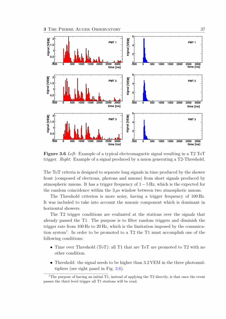
3 The Pierre Auger Observatory 37
sign
al [V
EM]
sign
al [V
EM]
sign
al [V
EM]
time [ns]
time [ns]
time [ns]
sign
al [V
EM]
sign
al [V
EM]
sign
al [V
EM]
time [ns]
time [ns]
time [ns]
Figure 3.6 Left: Example of a typical electromagnetic signal resulting in a T2 ToTtrigger. Right: Example of a signal produced by a muon generating a T2-Threshold.
The ToT criteria is designed to separate long signals in time produced by the shower
front (composed of electrons, photons and muons) from short signals produced by
atmospheric muons. It has a trigger frequency of 1− 5Hz, which is the expected for
the random coincidence within the 3µs window between two atmospheric muons.
The Threshold criterion is more noisy, having a trigger frequency of 100Hz.
It was included to take into account the muonic component which is dominant in
horizontal showers.
The T2 trigger conditions are evaluated at the stations over the signals that
already passed the T1. The purpose is to filter random triggers and diminish the
trigger rate from 100Hz to 20Hz, which is the limitation imposed by the comunica-
tion system1. In order to be promoted to a T2 the T1 must accomplish one of the
following conditions:
❼ Time over Threshold (ToT): all T1 that are ToT are promoted to T2 with no
other condition.
❼ Threshold: the signal needs to be higher than 3.2VEM in the three photomul-
tipliers (see right panel in Fig. 3.6).
1The purpose of having an initial T1, instead of applying the T2 directly, is that once the eventpasses the third level trigger all T1 stations will be read.

38 3.1 Surface Detector
If a signal satisfies both conditions it is labeled as ToT. Only when the station
has a T2, it sends the trigger (not the trace) information to the CDAS.
The T3 trigger conditions are applied in real time at the level of the global
detector. The CDAS monitors the stream of incoming T2 events with a software
on a central computer. The T2 events are stored in a temporary buffer and sorted
according to their trigger time. This buffer is then scanned with a sliding window
of 50µs in search of a compact spatial configuration of the T2-emmitting stations in
the window. The two possible conditions for a set of T2 stations producing a T3 in
the surface detector are:
❼ TOT2C1&3C2: Only ToT stations are considered. The compact spatial con-
figuration requires that one of the stations must have at least one neighbour
in the first crown and a second in the second crown (see left panel in Fig. 3.7).
Once the spatial coincidence is verified, timing criteria are imposed: each T2
must be within (6 + 5Cn)µs of the first one, where Cn denotes nth crown. .
❼ 2C1&3C2&4C4: The second T3 mode is more permissive. It requires a four-
fold coincidence of any T2 with a moderate compactness. Namely, among the
four fired stations at least one must have a neighbour in the the first crown,
another in the second and the last one can be as far as in the fourth (see
right panel in Fig. 3.7). Concerning timing criteria, the same logic as for the
“ToT2C1&3C2” is applied.
If any of those conditions is fullfilled, the central computer emits a T3.
Up to January 2007, the entire surface detector array was read out upon a T3
event. The SD array was still growing at that time up to a point, where the read-out
of the whole array produced an unacceptably high load on the radio communication
system. The CDAS was therfore changed and since then it reads out only the first
six crowns around each T2.
Upon a read-out request, every candidate station sends its station ID, signal
traces, trigger information, position, calibration histograms, and error code con-
cerning the communication to the CDAS.
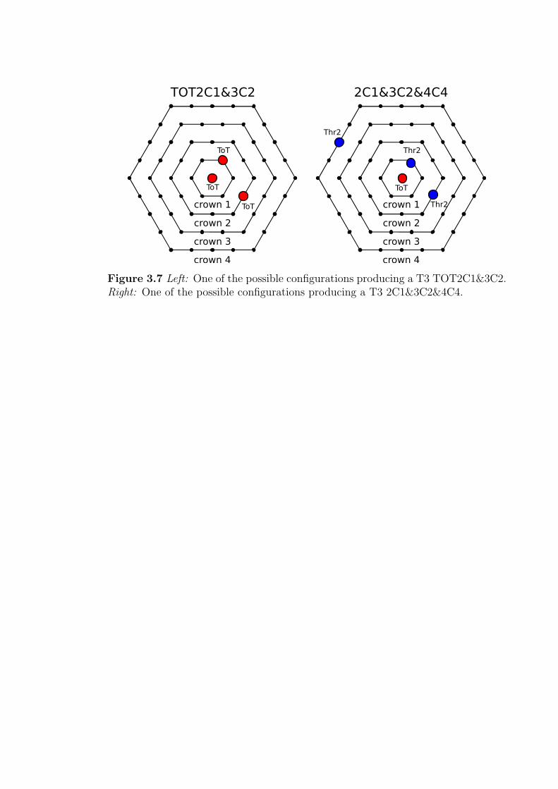
crown 1
crown 2
crown 3
crown 4
ToT
ToT
ToT
TOT2C1&3C2 2C1&3C2&4C4
crown 1
crown 2
crown 3
crown 4
ToT
Thr2
Thr2
Thr2
Figure 3.7 Left: One of the possible configurations producing a T3 TOT2C1&3C2.Right: One of the possible configurations producing a T3 2C1&3C2&4C4.

4Monte Carlo simulations:neutrinos
Monte Carlo (MC) simulations of neutrino interactions and neutrino-induced
showers are a fundamental tool in this thesis. Given the fact that there are no
neutrino induced showers detected until now, it is necessary to rely on simulations
for the development of the identification criteria and for the calculation of the surface
detector exposure to UHE neutrinos.
In Chapter 2 we have summarized the weak interaction channels through which a
neutrino can initiate an atmospheric shower. In this chapter we will concentrate on
the “Earth-skimming” channel and explain the simulation process. We will separate
this process into two steps:
1. Earth processes: neutrino interaction and tau propagation in the Earth crust
(Section 4.1).
2. Atmospheric processes: tau decay, atmospheric shower and particle detection
(Section 4.2).
In Section 4.3 we define a weight for each simulated shower to take into account
the probability to be produced by a diffuse isotropic E−2 neutrino flux.
4.1 Earth processes
In order to simulate the interactions of UHE ντ in the Earth, we have to charac-
terize the different physical processes at work in the neutrino and tau propagation.
41
42 4.1 Earth processes
4.1.1 Neutrino Interaction
During the propagation of the neutrino through the Earth, it will interact with
nucleons from the surrounding matter. The interaction with electrons is negligi-
ble1 [82]. In the framework of the Standard Model, the neutrino-nucleon charged
currrent (CC) (ντ +N → τ+X) and neutral current (NC) (ντ +N → ντ +X) cross-
sections, σCCντ and σNC
ντ , describe deep-inelastic scattering (DIS) processes. The X
stands for all the resulting particles disregarding the τ (ντ ) in the CC (NC) process
which result in a jet.
The cross-sections are expressed in terms of the structure functions of the nu-
cleon, which in turn depend on the individual parton distribution functions (PDFs).
The PDFs are obtained from measurements at accelerators, in restricted ranges of
Bjorken-x and momentum transfer Q2. However, the kinematic range probed by
UHE neutrinos is outside the measured domain and therefore extrapolations are
needed. If a neutrino interacts with a nucleon at a center of mass energy√s = 1014
eV (Eν = 5.3× 10¹⁸ eV) the relevant range of x is: 10−8 . x . 10−4. The relevant
range in Q2 is: 50 . Q2 . 104 GeV2, where the exact region increases only slowly
with Eν because the contribution of higher Q2 (Q2 > M2W ) is suppressed by the
W -propagator.
The calculation of the σντ at energies above 1017 eV has been performed by
several authors. Pioneering estimates were presented in 1996 by Gandhi et al us-
ing PDFs from the CTEQ and MRS collaborations and applying a leading-order
(LO) Altarelli-Parisi evolution to obtain the distributions at high Q2 [82]. More
recently, between 2006 and 2011, Sarkar et al updated the result using new HERA
data which modified the PDFs and also extended the calculation at next-to-leading-
order (NLO) [97, 98]. We adopt this result as the reference cross-section used in
this work. In 2008, Armesto et al studied different methods to calculate the σντ
in order to estimate the uncertainty of this magnitude [99]. The uncertainty is
dominated by the way the PDFs are extrapolated to very low x. The highest es-
timate of σντ was derived extrapolating the structure function as F2 ∝ x−λ with
λ = 0.0481 ln(Q/0.0292)2 saturating at λ = 0.4 as higher values of λ are in contra-
diction with perturbative calculations. The lowest σντ estimate was derived using an
extrapolation of F2 following the ASW parametrization which saturates faster [100].
In Figure 4.1 we show the three calculations for the σCCντ described before together
with the relative difference between the highest (lowest) and the reference 2. Similar
considerations apply to the neutral current channel, which is ∼ 2.5 lower than the
CC case.
1The σ(ντe) is 0.01 that of σ(ντN).2The relative difference for a given model A is A−Ref
Ref
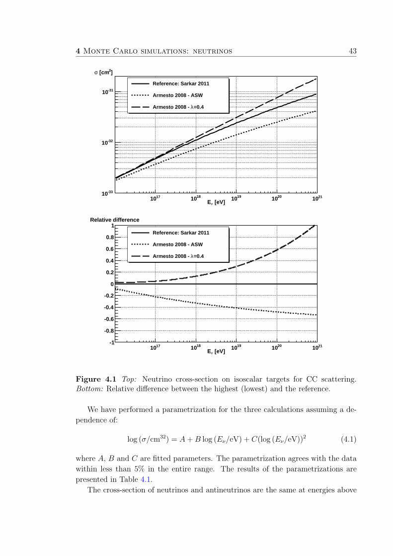
4 Monte Carlo simulations: neutrinos 43
[eV]νE1710 1810 1910 2010 2110
-3310
-3210
-3110
]2 [cmσ
Reference: Sarkar 2011
Armesto 2008 - ASW
=0.4λArmesto 2008 -
[eV]νE1710 1810 1910 2010 2110
-1
-0.8
-0.6
-0.4
-0.2
0
0.2
0.4
0.6
0.8
1Relative difference
Reference: Sarkar 2011
Armesto 2008 - ASW
=0.4λArmesto 2008 -
Figure 4.1 Top: Neutrino cross-section on isoscalar targets for CC scattering.Bottom: Relative difference between the highest (lowest) and the reference.
We have performed a parametrization for the three calculations assuming a de-
pendence of:
log (σ/cm32) = A+B log (Eν/eV) + C(log (Eν/eV))2 (4.1)
where A, B and C are fitted parameters. The parametrization agrees with the data
within less than 5% in the entire range. The results of the parametrizations are
presented in Table 4.1.
The cross-section of neutrinos and antineutrinos are the same at energies above

44 4.1 Earth processes
Model A B C
Reference: Sarkar 2011 -0.39 0.64 -0.016Highest (optimistic): pQCD λ = 0.4 0.27 0.45 -0.003Lowest (pesimistic): ASW 0.25 0.52 -0.013
Table 4.1 Parameters in equation 4.1 for the three models described in the text.
1017 eV. At 1014 eV the neutrino cross-section is higher by only 15%. This means
that we can consider only neutrino cross-sections and use the same results for the
antineutrinos.
Another important parameter when considering the DIS processes is the distri-
bution of the energy transfered to the jet in an interaction. This magnitude is called
the inelasticity y. In Figure 4.2 we show the distribution of the inelasticity for CC
and NC channels for an interaction of a 1018 eV neutrino with an isoscalar target.
The average inelasticity is ∼ 0.2 for both CC and NC processes. This distribution
also does not change when considering antineutrinos and remains the same at higher
energies.
Inelasticity
Figure 4.2 Inelasticity distribution for the charged and neutral interactions of a1018 eV neutrino and an isoscalar target.
4.1.2 Tau Propagation
There are different processes through which the tau can loose energy as it prop-
agates through the Earth. The four dominant ones are ionization, bremsstrahlung,
4 Monte Carlo simulations: neutrinos 45
pair production and photonuclear effect.
To first order energy loss by ionization is independent of the τ energy, while the
other three processes are linear in E. For this reason the energy loss per unit length
can be written as:
−⟨dE
dX
⟩
= α(E) + β(E)× E (4.2)
α(E) and β(E) are functions of the energy and describe the deviations from the first
order behaviour. α(E) represents the ionization losses and β(E) = βbremss(E) +
βpair(E) + βnuc(E), where the suffixes stand for the different electromagentic pro-
cesses, bremsstrahlung (brem), pair production (pair) and photonuclear effect (nuc).
Ionization is produced by the coulomb interaction of the τ with the electrons
in the medium. This process is described by the Bethe-Bloch equation, with a
correction for density effects, which comes from the fact that, in a dense medium like
Earth, atoms cannot be considered isolated. For the range of energies considered in
this work, the effect of ionization is negligible compared to the three other processes:
−⟨dE
dX
⟩
∼ 10−3 GeV g−1cm2 (4.3)
Between 1020 eV and 1016 eV the increase of the energy loss due to ionization is only
30% 3.
The evaluation of bremsstrahlung and pair-production tau energy loss is carried
in detail in Ref [101] based on the differential bremsstrahlung cross-section devel-
oped by Petrukhin and Shestakov [102] and pair production differential cross-section
estimation from Kokoulin and Petrukhin [103].
For muons, bremsstrahlung is a dominant source of energy loss, but for tau lep-
tons it appears highly suppressed by a(
mµ
mτ
)2
factor, where mτ ≈ 17×mµ ≈ 3500×me. For the range of energies considered in this work, the effect of bremsstrahlung
large compared to ionization:
−⟨dE
dX
⟩
bremss
∼ 8× 10⁻⁹ × E g−1cm2 (4.4)
βbremss(E) can be considered constant in the entire range.
For pair-production the energy dependence is also negligible:
−⟨dE
dX
⟩
∼ 1.4× 10⁻⁷ × E g−1cm2 (4.5)
It is more important than bremsstrahlung by a factor 175, so bremsstrahlung can
also be ignored.
3 α(1020eV)
α(1016eV)∼ 1.3
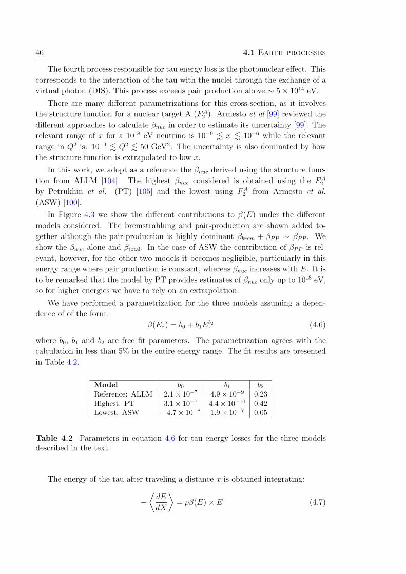
46 4.1 Earth processes
The fourth process responsible for tau energy loss is the photonuclear effect. This
corresponds to the interaction of the tau with the nuclei through the exchange of a
virtual photon (DIS). This process exceeds pair production above ∼ 5× 10¹⁴ eV.
There are many different parametrizations for this cross-section, as it involves
the structure function for a nuclear target A (FA2 ). Armesto et al [99] reviewed the
different approaches to calculate βnuc in order to estimate its uncertainty [99]. The
relevant range of x for a 1018 eV neutrino is 10−9 . x . 10−6 while the relevant
range in Q2 is: 10−1 . Q2 . 50 GeV2. The uncertainty is also dominated by how
the structure function is extrapolated to low x.
In this work, we adopt as a reference the βnuc derived using the structure func-
tion from ALLM [104]. The highest βnuc considered is obtained using the FA2
by Petrukhin et al. (PT) [105] and the lowest using FA2 from Armesto et al.
(ASW) [100].
In Figure 4.3 we show the different contributions to β(E) under the different
models considered. The bremstrahlung and pair-production are shown added to-
gether although the pair-production is highly dominant βbrem + βPP ∼ βPP . We
show the βnuc alone and βtotal. In the case of ASW the contribution of βPP is rel-
evant, however, for the other two models it becomes negligible, particularly in this
energy range where pair production is constant, whereas βnuc increases with E. It is
to be remarked that the model by PT provides estimates of βnuc only up to 1018 eV,
so for higher energies we have to rely on an extrapolation.
We have performed a parametrization for the three models assuming a depen-
dence of of the form:
β(Eτ ) = b0 + b1Eb2τ (4.6)
where b0, b1 and b2 are free fit parameters. The parametrization agrees with the
calculation in less than 5% in the entire energy range. The fit results are presented
in Table 4.2.
Model b0 b1 b2Reference: ALLM 2.1× 10⁻⁷ 4.9× 10⁻⁹ 0.23Highest: PT 3.1× 10⁻⁷ 4.4× 10⁻¹⁰ 0.42Lowest: ASW −4.7× 10⁻⁸ 1.9× 10⁻⁷ 0.05
Table 4.2 Parameters in equation 4.6 for tau energy losses for the three modelsdescribed in the text.
The energy of the tau after traveling a distance x is obtained integrating:
−⟨dE
dX
⟩
= ρβ(E)× E (4.7)
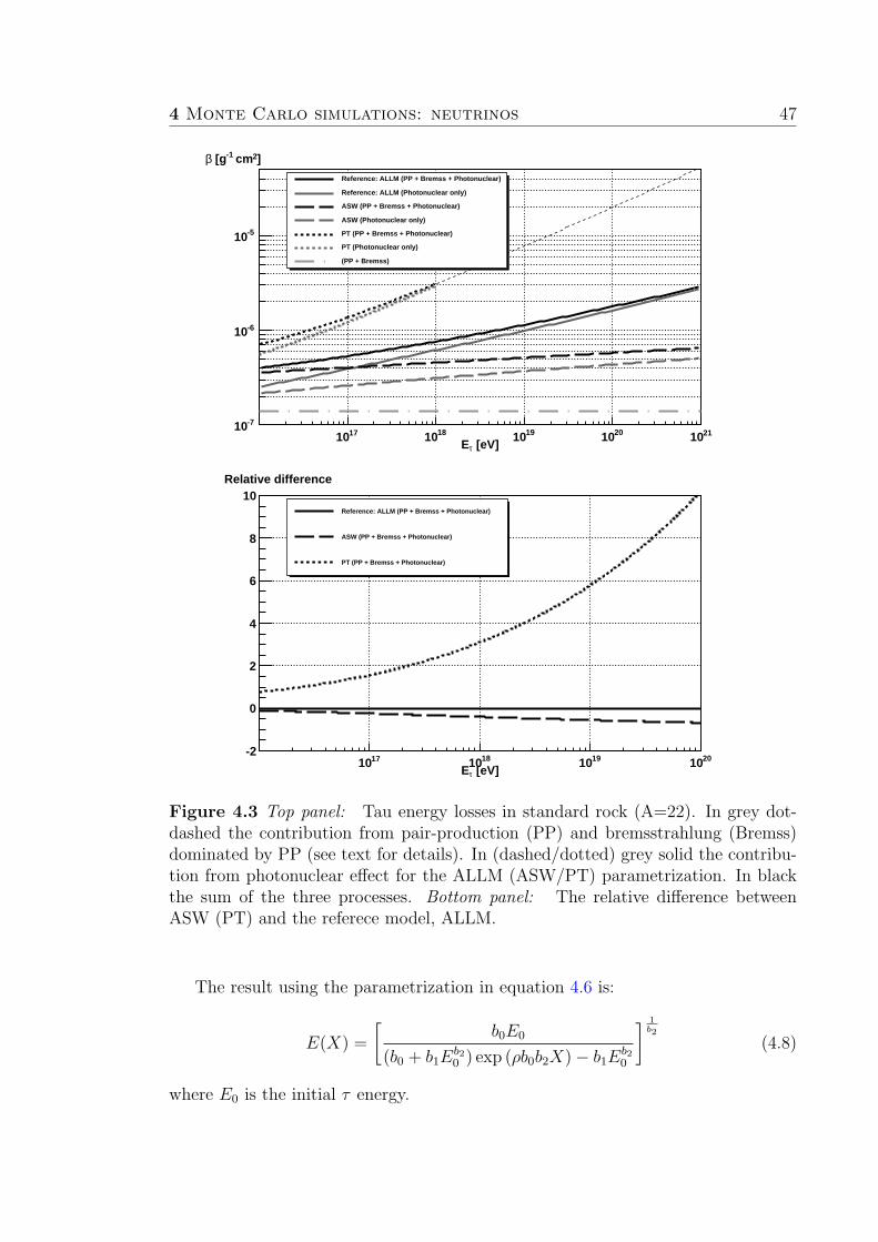
4 Monte Carlo simulations: neutrinos 47
[eV]τE1710 1810 1910 2010 2110
-710
-610
-510
]2 cm-1 [gβReference: ALLM (PP + Bremss + Photonuclear)
Reference: ALLM (Photonuclear only)
ASW (PP + Bremss + Photonuclear)
ASW (Photonuclear only)
PT (PP + Bremss + Photonuclear)
PT (Photonuclear only)
(PP + Bremss)
[eV]τE1710 1810 1910 2010
-2
0
2
4
6
8
10Relative difference
Reference: ALLM (PP + Bremss + Photonuclear)
ASW (PP + Bremss + Photonuclear)
PT (PP + Bremss + Photonuclear)
Figure 4.3 Top panel: Tau energy losses in standard rock (A=22). In grey dot-dashed the contribution from pair-production (PP) and bremsstrahlung (Bremss)dominated by PP (see text for details). In (dashed/dotted) grey solid the contribu-tion from photonuclear effect for the ALLM (ASW/PT) parametrization. In blackthe sum of the three processes. Bottom panel: The relative difference betweenASW (PT) and the referece model, ALLM.
The result using the parametrization in equation 4.6 is:
E(X) =
[b0E0
(b0 + b1Eb20 ) exp (ρb0b2X)− b1E
b20
] 1b2
(4.8)
where E0 is the initial τ energy.

48 4.1 Earth processes
The τ is a particle with a short lifetime (ττ = 2.9 × 10⁻¹³s, cττ = 87µm). The
decay length is λdec = c ττEτ
mτ≈ 49
(Eτ
1018eV
)km. At low energies the tau decay length
is small enough so that energy losses can be neglected. However, in the range of
energies considered in this work (E > 1016.5eV) this is not the case. The survival
probability as a function of distance X is given by:
P (X) = exp
[
−∫ X
0
mτ
cττ
dX
E(X)
]
(4.9)
If no energy losses are considered the result for a τ with an initial energy E0 is
straightforward: P (x) = exp
(
−mτX
cττE0
)
= exp
(
− X
λdec
)
. When tau energy losses
are taken into account we have to integrate equation 4.8.
The range R is defined as the distance a beam traverses before its inelasticity is
reduced to 1/e, i.e. P (R) = e−1. In Figure 7.13 we show the range as a function of
the initial energy of the τ .
Even though the range decreases when the tau energy loss increases the realation
between the two is not inversely proportional. For example, at 1020 eV PT is 11
times higher than ALLM, while the range is only 3 times lower.
Now we can estimate the probability that a 1 Earth-skimming neutrino will give
rise to an emerging tau. Given that the interaction length, λint, for a 1018 eV tau
neutrino in rock is 620 km, and that at 1 the distance through Earth is 220 km,
only 30% of the incident neutrinos will interact. Figure 4.5 shows the interaction
probability density as a function of travelled distance. Now, 1018 eV interacting
neutrinos will produce taus with average energy of 8× 10¹⁷ eV, which have a 12 km
range in rock. Therefore, only the neutrinos interacting in the last 12 km of their
journey through Earth will produce an emerging tau. These are signaled by the
black area on Figure 4.5, and correspond to 1.4% (4.6%) of the incident (interacting)
neutrinos.
4.1.3 Monte Carlo simulations
The Monte Carlo generator provides a natural way to deal with both neutrino
interactions and tau energy losses. The method consists in following the incident
particles all the way through the rock, deciding at each step on their fate accord-
ing to the distribution of possible processes. The algorithm used is schematically
represented in Figure 4.6.
Using this MC generator with a fixed neutrino energy and angle of incidence 4,
one obtains the energy probability density for producing a tau that reaches the
surface of the Earth dnτ
d logEτ. To a very good approximation the angle of incidence
4The angle of incidence fixes the amount of matter the particles traverse.
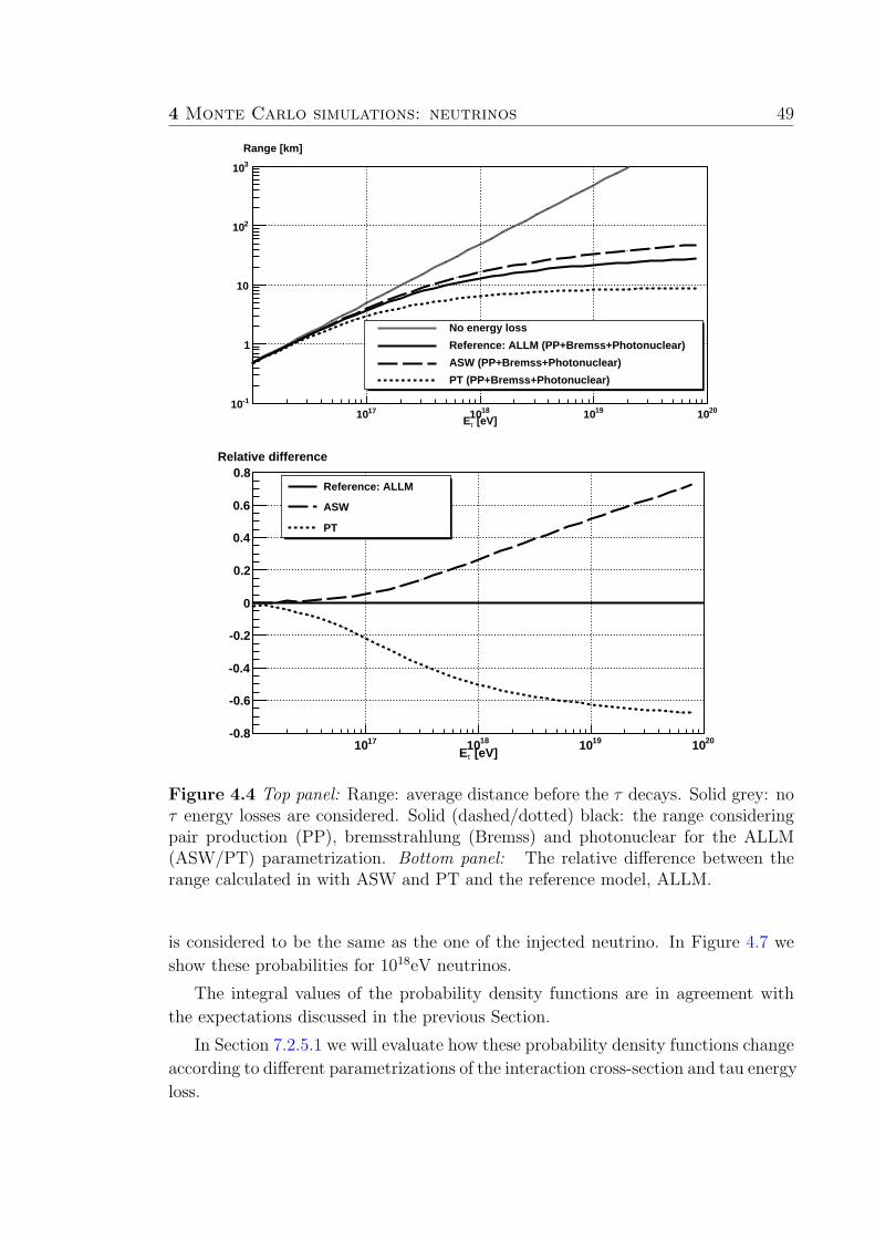
4 Monte Carlo simulations: neutrinos 49
[eV]τE1710 1810 1910 2010
-110
1
10
210
310
Range [km]
No energy loss
Reference: ALLM (PP+Bremss+Photonuclear)
ASW (PP+Bremss+Photonuclear)
PT (PP+Bremss+Photonuclear)
[eV]τE1710 1810 1910 2010
-0.8
-0.6
-0.4
-0.2
0
0.2
0.4
0.6
0.8Relative difference
Reference: ALLM
ASW
PT
Figure 4.4 Top panel: Range: average distance before the τ decays. Solid grey: noτ energy losses are considered. Solid (dashed/dotted) black: the range consideringpair production (PP), bremsstrahlung (Bremss) and photonuclear for the ALLM(ASW/PT) parametrization. Bottom panel: The relative difference between therange calculated in with ASW and PT and the reference model, ALLM.
is considered to be the same as the one of the injected neutrino. In Figure 4.7 we
show these probabilities for 1018eV neutrinos.
The integral values of the probability density functions are in agreement with
the expectations discussed in the previous Section.
In Section 7.2.5.1 we will evaluate how these probability density functions change
according to different parametrizations of the interaction cross-section and tau energy
loss.
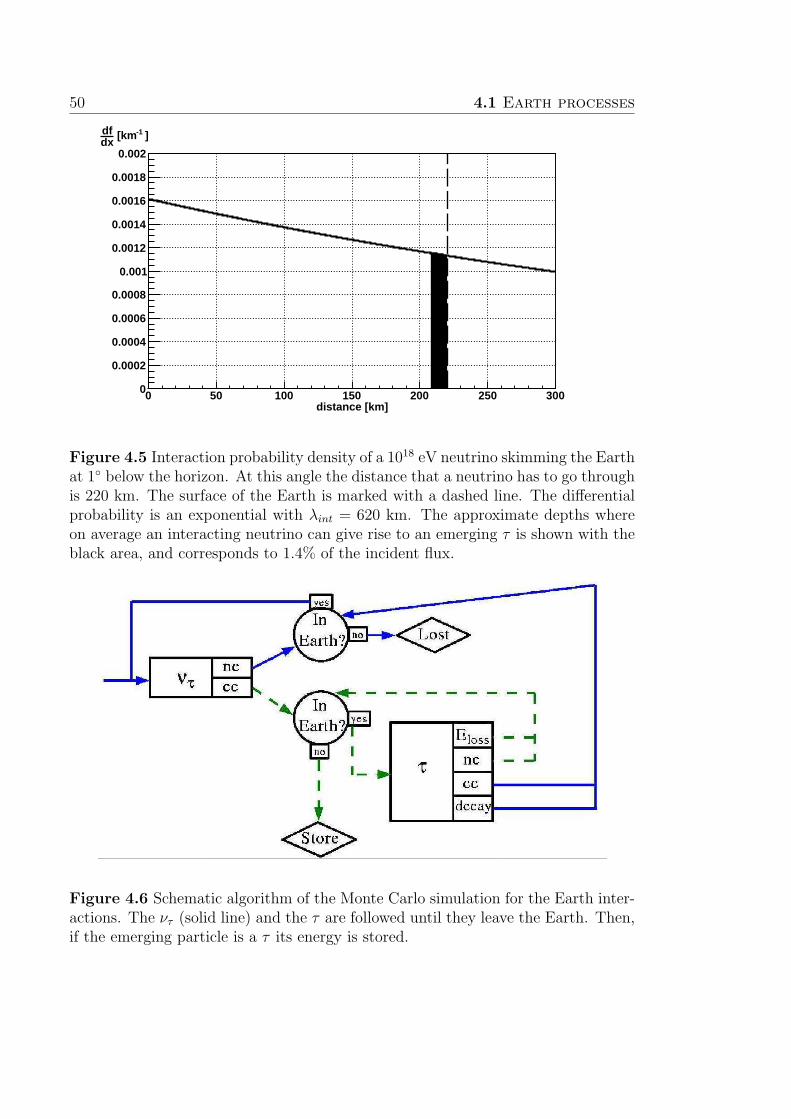
50 4.1 Earth processes
distance [km]0 50 100 150 200 250 3000
0.0002
0.0004
0.0006
0.0008
0.001
0.0012
0.0014
0.0016
0.0018
0.002
]-1 [kmdxdf
Figure 4.5 Interaction probability density of a 1018 eV neutrino skimming the Earthat 1 below the horizon. At this angle the distance that a neutrino has to go throughis 220 km. The surface of the Earth is marked with a dashed line. The differentialprobability is an exponential with λint = 620 km. The approximate depths whereon average an interacting neutrino can give rise to an emerging τ is shown with theblack area, and corresponds to 1.4% of the incident flux.
Figure 4.6 Schematic algorithm of the Monte Carlo simulation for the Earth inter-actions. The ντ (solid line) and the τ are followed until they leave the Earth. Then,if the emerging particle is a τ its energy is stored.

4 Monte Carlo simulations: neutrinos 51
16 16.2 16.4 16.6 16.8 17 17.2 17.4 17.6 17.8 180
0.002
0.004
0.006
0.008
0.01
0.012
0.014
τ E10
dlogτdn
/eVτ E10
log
=90.683θ
=91.827θ
=92.972θ
Figure 4.7 Probability density function (pdf) for an emerging tau as a functionof its energy in logarithmic scale. The pdf depends on the energy of the neutrinoand the zenith angle θ. In this example the energy is fixed at Eν = 1018 eV. Threezenith angles are shown: θ = 90.683 (circles), θ = 91.827 (squares) and θ = 92.972
(triangles) with corresponding traveled distances in the of Earth 152, 407 and 661km. The integral of each pdf is 1.3%, 0.8% and 0.5% respectively.
4.2 Atmospheric simulation
The simulation sequence in the atmosphere can be divided into three steps:
1. τ decay: Determination of the particles produced when the τ decays (Sec. 4.2.1).
2. Atmospheric evolution of the shower: simulation of the shower generated
by the τ decay products until the shower reaches the surface of the Earth
(Sec. 4.2.2).
3. Surface detector response: Simulation of the signals registered by the
surface detector stations of the Pierre Auger Observatory from the particles
that go through them (Sec. 4.2.3).
The sequence is schematically represented in Figure 4.8.

52 4.2 Atmospheric simulation
2. AIRES
3. GEANT 4
τ
1. TAUOLA
Decayproducts
Figure 4.8 Scheme of the three different processes taken into accout for the simu-lation of the atmospheric and detector simulation. In green the high energy τ decay,in blue the atmospheric evolution of the shower and in red the surface detectorresponse.
4.2.1 Simulation of τ decay
The CC interaction that gives rise to τ leptons is mediated through theW boson.
The W couples only to left chirality and at ultra-relativistic energies chirality is the
same as helicity. Consequently, tau neutrinos ντ (tau anti-neutrinos ντ ) will produce
only τ− with negative helicity (τ+ with positive helicity), Figure 4.9.
Figure 4.9 Feynman diagrams of the ντ and ντ interactions resulting in a taulepton.
In order to simulate the decay of the tau we use the package TAUOLA [106] that
contains all the experimental information on final states and branching ratios. In
Table 4.3 we show the most important channels.
It is important to use only negative helicity for the τ− decay. The fraction of
energy that goes into the shower, i.e the sum of the energy of all particles except
for neutrinos, can change considerably if one incorrectly uses positive polarization
for negative taus. In order to illustrate this we can consider channel number 4 in
Table 4.3, which provides a simple example.

4 Monte Carlo simulations: neutrinos 53
Number Decay Probability (%)1 τ− → π−π0ντ ∼25.52 τ− → e−νeντ ∼17.93 τ− → µ−νµντ ∼17.4 Unobservable4 τ− → π−ντ ∼10.95 τ− → 2π−π+ντ ∼9.36 τ− → π−2π0ντ ∼9.37 τ− → 2π−π+π0ντ ∼4.68 τ− → π−3π0ντ ∼1.0
Table 4.3 The eight most frequent τ decay channels. The other decay channelsamount to 4.1%. τ+ decay modes are charge conjugate of the modes shown. Channelnumber 3 is unobservable because the µ is unlikely to interact or decay and producean UHE shower within the observable region of the atmosphere.
Consider the τ−− → π− + ντ decay in the Laboratory frame choosing the z-axis
parallel to the τ momentum. The energy of the particles is:
ELabi = γ(ECM
i + βpCMz,i ) (4.10)
where i = τ, ν and π−, γ = (1 − β2)−1 = ELabτ
mτand pz is the component of the
momentum parallel to the direction of the τ .
For ELabτ ∼ 1018eV and mτ = 1.77 GeV, γ ≫ 1 so β ≈ 1 and the fraction of
energy that goes into the shower is:
xi =ELab
π−
ELabτ
=ECM
π−+ βpCM
z,π−
ECMτ + βpCM
z,τ
=1
2(1 + cosΘ) (4.11)
where Θ is the angle between the polarization of the τ and ~p CMπ−
.
For a τ polarized in z the distribution of the parallel component of the π− is
shown in Figure 4.10. The τ− with negative (positive) helicity favours π− produced
in the backward (forward) direction. The result is that the fraction of energy that
goes into the shower (the energy of the π−) is less for τs with negative helicity.
The differences between using negative and positive helicity are shown in Fi-
gure 4.11 when considering all channels and the corresponding branching ratios..
Using unpolarized or positive helicity for the τ− results in an overestimation of the
exposure.
It is important to notice that the distribution shown in Figure 4.11 is the same
for τ+ with positive polarization. In this way, one can perform the simulations only
with τ− decays, which are the result of the neutrino DIS, and they will also apply
to the case of antineutrinos cosmic rays.
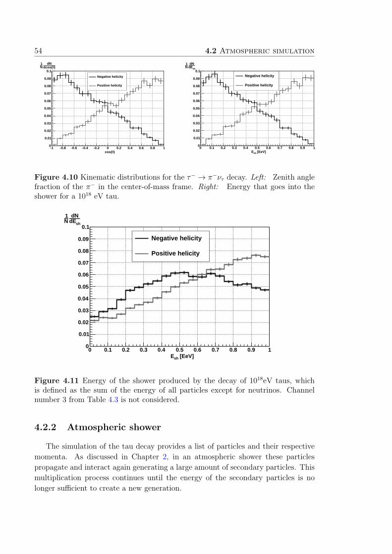
54 4.2 Atmospheric simulation
-1 -0.8 -0.6 -0.4 -0.2 0 0.2 0.4 0.6 0.8 10
0.01
0.02
0.03
0.04
0.05
0.06
0.07
0.08
0.09
0.1)θdcos(
dN N1
)θcos(
Negative helicity
Positive helicity
0 0.1 0.2 0.3 0.4 0.5 0.6 0.7 0.8 0.9 10
0.01
0.02
0.03
0.04
0.05
0.06
0.07
0.08
0.09
0.1shdE
dN N1
[EeV]shE
Negative helicity
Positive helicity
Figure 4.10 Kinematic distributions for the τ− → π−ντ decay. Left: Zenith anglefraction of the π− in the center-of-mass frame. Right: Energy that goes into theshower for a 1018 eV tau.
0 0.1 0.2 0.3 0.4 0.5 0.6 0.7 0.8 0.9 10
0.01
0.02
0.03
0.04
0.05
0.06
0.07
0.08
0.09
0.1shdE
dN N1
[EeV]shE
Negative helicity
Positive helicity
Figure 4.11 Energy of the shower produced by the decay of 1018eV taus, whichis defined as the sum of the energy of all particles except for neutrinos. Channelnumber 3 from Table 4.3 is not considered.
4.2.2 Atmospheric shower
The simulation of the tau decay provides a list of particles and their respective
momenta. As discussed in Chapter 2, in an atmospheric shower these particles
propagate and interact again generating a large amount of secondary particles. This
multiplication process continues until the energy of the secondary particles is no
longer sufficient to create a new generation.
4 Monte Carlo simulations: neutrinos 55
In order to simulate this process it is necessary to count with a detailed knowledge
of all possible interactions a particle may suffer during the evolution of the shower.
This is a complex problem which requires the use of different tools including models
of hadronic interactions and the description of the atmospheric density as a function
of the altitude.
There are a variety of software packages which group these tools and allow to
consider all the aspects of the simulation of an atmospheric shower. The two most
common packages are CORSIKA [107] and AIRES [108] which present similar char-
acteristics. In this work, we used AIRES as CORSIKA still has no implementation
for up-going showers. A computer code was developed to interpret the TAUOLA
output and incorporate the particles within the framework of AIRES. For each of
the particles, this code also sets the angle, time and injection depth.
The first generation of particles can have energies four orders of magnitud higher
than the ones achieved today in accelerator experiments. Consequently, the models
used to simulate the interactions during the first steps of the shower are necessarily
extrapolations of measurements performed at much lower energies. As the astropar-
ticle community has not reached consensus about which is the best hadronic model,
the AIRES package incorporates the most common ones: SIBYLL [109], QGSJET-
I [110] and QGSJET-II [111]. In this work we decided to use the last one to have
consistency with the downward-going neutrino analysis in [75]. In Section 7.2.5.2
we discuss the estimation of the uncertainty associated to this choice.
The time and computer memory required to simulate an atmospheric shower
scales with the number of particles generated during its evolution. At energies of
the order of the EeV this number can be superior to 1010 particles so the simulation
of the trajectory and their individual evolution is impossible.
Instead, one uses a statistical sampling method in which only a small represen-
tative fraction of the particles is propagated. A weight is assigned to each of them
to compensate for those particles that are not followed. This method is known as
“thinning” [112]. During the first steps of the simulation all propagated particles
have a weight of 1. When the multiplicity of the shower increases, only a small
fraction of the particles is simulated in detail and their weight increases. The idea
of the thinning method is ilustrated considering the following process:
A → B1, B2, . . . , Bn with n ≥ 1 (4.12)
where a “primary” particle A generates a set of secondaries B1, B2, . . . , Bn.
Let us denote EA (EBi) the energy of A (Bi), and consider a fixed thinning energy
Eth. Before incorporating the secondaries to the simulation processes, the energy is
compared with Eth and:
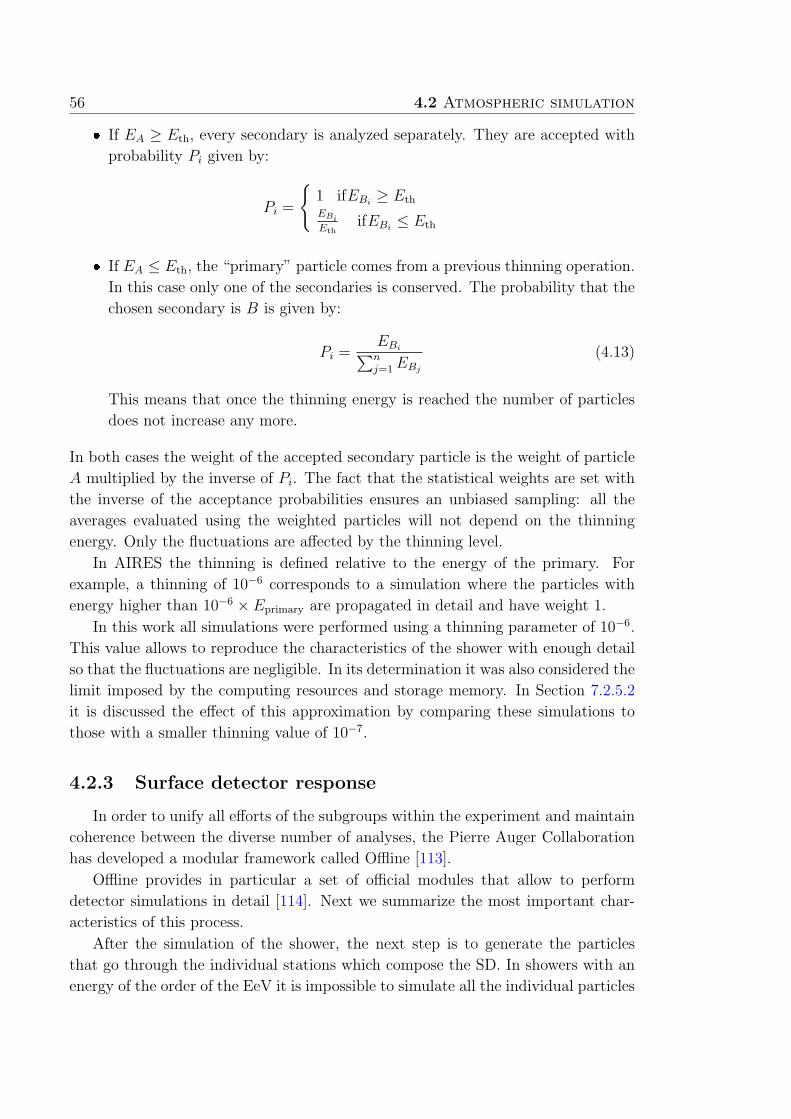
56 4.2 Atmospheric simulation
❼ If EA ≥ Eth, every secondary is analyzed separately. They are accepted with
probability Pi given by:
Pi =
1 ifEBi≥ Eth
EBi
EthifEBi
≤ Eth
❼ If EA ≤ Eth, the “primary” particle comes from a previous thinning operation.
In this case only one of the secondaries is conserved. The probability that the
chosen secondary is B is given by:
Pi =EBi
∑nj=1 EBj
(4.13)
This means that once the thinning energy is reached the number of particles
does not increase any more.
In both cases the weight of the accepted secondary particle is the weight of particle
A multiplied by the inverse of Pi. The fact that the statistical weights are set with
the inverse of the acceptance probabilities ensures an unbiased sampling: all the
averages evaluated using the weighted particles will not depend on the thinning
energy. Only the fluctuations are affected by the thinning level.
In AIRES the thinning is defined relative to the energy of the primary. For
example, a thinning of 10−6 corresponds to a simulation where the particles with
energy higher than 10−6 × Eprimary are propagated in detail and have weight 1.
In this work all simulations were performed using a thinning parameter of 10−6.
This value allows to reproduce the characteristics of the shower with enough detail
so that the fluctuations are negligible. In its determination it was also considered the
limit imposed by the computing resources and storage memory. In Section 7.2.5.2
it is discussed the effect of this approximation by comparing these simulations to
those with a smaller thinning value of 10−7.
4.2.3 Surface detector response
In order to unify all efforts of the subgroups within the experiment and maintain
coherence between the diverse number of analyses, the Pierre Auger Collaboration
has developed a modular framework called Offline [113].
Offline provides in particular a set of official modules that allow to perform
detector simulations in detail [114]. Next we summarize the most important char-
acteristics of this process.
After the simulation of the shower, the next step is to generate the particles
that go through the individual stations which compose the SD. In showers with an
energy of the order of the EeV it is impossible to simulate all the individual particles

4 Monte Carlo simulations: neutrinos 57
and just a representative sample is simulated (see Sec. 4.2.2). For this reason, the
first step is to perform an “unthinning”: a statistical regeneration of the particles
to estimate which are the ones entering the SD stations. In this work a technique
based on the procedure described in [115] was used, adapted so that one can treat
very inclined showers.
Once that the particles that go through the stations are defined, a simulation
based on GEANT4 [116] is used to describe the production and propagation of
Cherenkov photons within the stations. Each of these photons is propagated until
it reaches one of the PMTs or is absorbed in the water. Next, a PMT and electronic
dedicated simulation is used to transform these photons into the signal registered
by each station.
The simulated signals in the three PMTs are used to calculate the trigger level
of each station (ToT, Thr2, Thr1 or none). Those that do not reach any of the
trigger conditions are ignored. The stations with trigger level ToT or Thr2 are used
in the evaluation of the central trigger T3 (see Sec. 3.1.2). If the configuration of the
triggered stations does not produce a T3 trigger the event is discarded as it would
in the case of a real shower not triggering the SD.
4.3 Weights
As stated at the begining of this chapter, there are no neutrino induced showers
detected until now, so it is necessary to rely on simulations for the development of
the identification criteria and for the calculation of the exposure of the detector.
We have simulated 150 tau-induced showers for every point in Figure 4.12. A
point is defined by the tau energy Eτ , the zenith angle θ and the decay height Xd.
For each of the 150 cases the azimuth angle φ of the tau is extracted from a uniform
distribution.
Each of these points correspond to different situations which should not appear
with the same frequency in the simulated data because they have different probabil-
ities to be produced by a diffuse isotropic E−2 neutrino flux and to trigger the array.
For this reason, it is necessary to assign to each event a weight wi which takes into
account the contribution of that point to the number of expected events. We define
wi as the number of triggered simulated events per unit time and area for a diffuse
neutrino flux that decreases with energy as E−2ν .
In order to construct the weight, let us consider the ingredients needed to obtain
the expected number of events per unit time and area, dNexp
dtdA:
dNexp
dtdA=
∫
dEν
∫
dEτ
∫
dΩ
∫
dXd Φ(Eν) f(Eτ |θ, Eν)h(Xd|Eτ , θ)| cos θ| ε(Eτ , θ,Xd)
(4.14)
where we will assume Φ(Eν) = k E−2ν , with k the unknown normalization of the flux.
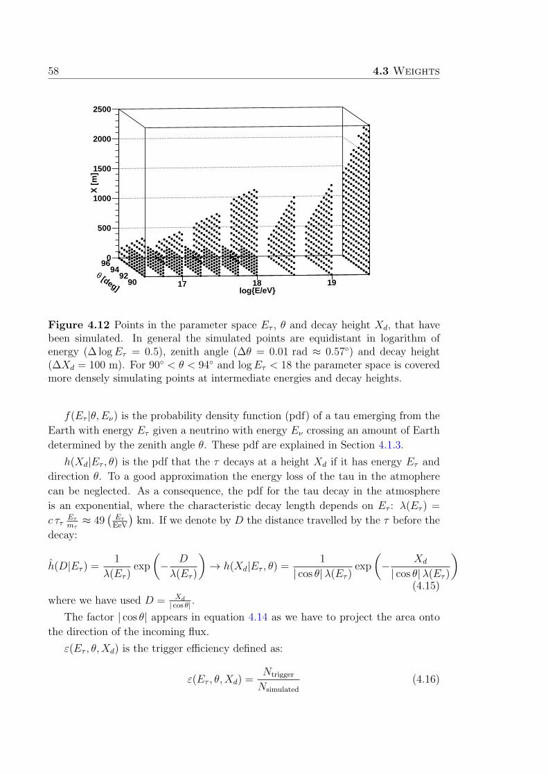
58 4.3 Weights
logE/eV17 18 19
[deg]
θ90
9294
96
X [
m]
0
500
1000
1500
2000
2500
Figure 4.12 Points in the parameter space Eτ , θ and decay height Xd, that havebeen simulated. In general the simulated points are equidistant in logarithm ofenergy (∆ logEτ = 0.5), zenith angle (∆θ = 0.01 rad ≈ 0.57) and decay height(∆Xd = 100 m). For 90 < θ < 94 and logEτ < 18 the parameter space is coveredmore densely simulating points at intermediate energies and decay heights.
f(Eτ |θ, Eν) is the probability density function (pdf) of a tau emerging from the
Earth with energy Eτ given a neutrino with energy Eν crossing an amount of Earth
determined by the zenith angle θ. These pdf are explained in Section 4.1.3.
h(Xd|Eτ , θ) is the pdf that the τ decays at a height Xd if it has energy Eτ and
direction θ. To a good approximation the energy loss of the tau in the atmophere
can be neglected. As a consequence, the pdf for the tau decay in the atmosphere
is an exponential, where the characteristic decay length depends on Eτ : λ(Eτ ) =
c ττEτ
mτ≈ 49
(Eτ
EeV
)km. If we denote by D the distance travelled by the τ before the
decay:
h(D|Eτ ) =1
λ(Eτ )exp
(
− D
λ(Eτ )
)
→ h(Xd|Eτ , θ) =1
| cos θ|λ(Eτ )exp
(
− Xd
| cos θ|λ(Eτ )
)
(4.15)
where we have used D = Xd
| cos θ|.
The factor | cos θ| appears in equation 4.14 as we have to project the area onto
the direction of the incoming flux.
ε(Eτ , θ,Xd) is the trigger efficiency defined as:
ε(Eτ , θ,Xd) =Ntrigger
Nsimulated
(4.16)
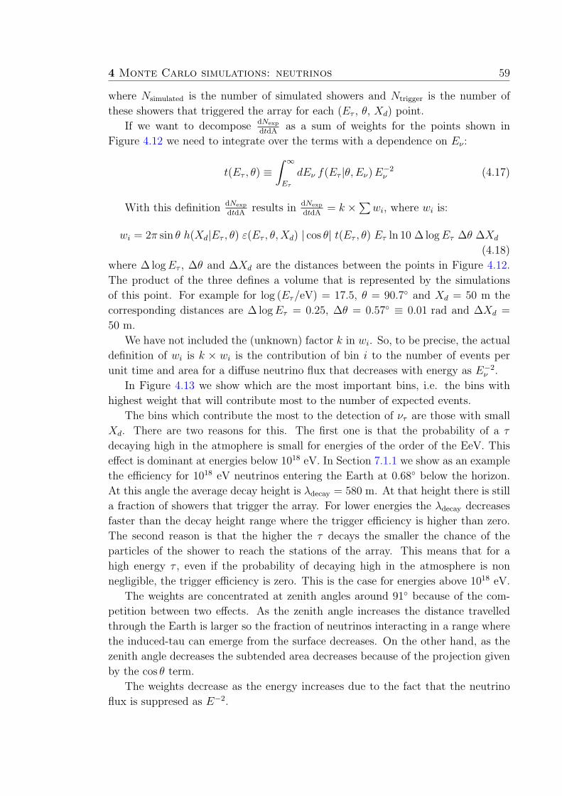
4 Monte Carlo simulations: neutrinos 59
where Nsimulated is the number of simulated showers and Ntrigger is the number of
these showers that triggered the array for each (Eτ , θ, Xd) point.
If we want to decompose dNexp
dtdAas a sum of weights for the points shown in
Figure 4.12 we need to integrate over the terms with a dependence on Eν :
t(Eτ , θ) ≡∫ ∞
Eτ
dEν f(Eτ |θ, Eν)E−2ν (4.17)
With this definition dNexp
dtdAresults in dNexp
dtdA= k ×∑
wi, where wi is:
wi = 2π sin θ h(Xd|Eτ , θ) ε(Eτ , θ,Xd) | cos θ| t(Eτ , θ) Eτ ln 10 ∆ logEτ ∆θ ∆Xd
(4.18)
where ∆ logEτ , ∆θ and ∆Xd are the distances between the points in Figure 4.12.
The product of the three defines a volume that is represented by the simulations
of this point. For example for log (Eτ/eV) = 17.5, θ = 90.7 and Xd = 50 m the
corresponding distances are ∆ logEτ = 0.25, ∆θ = 0.57 ≡ 0.01 rad and ∆Xd =
50 m.
We have not included the (unknown) factor k in wi. So, to be precise, the actual
definition of wi is k × wi is the contribution of bin i to the number of events per
unit time and area for a diffuse neutrino flux that decreases with energy as E−2ν .
In Figure 4.13 we show which are the most important bins, i.e. the bins with
highest weight that will contribute most to the number of expected events.
The bins which contribute the most to the detection of ντ are those with small
Xd. There are two reasons for this. The first one is that the probability of a τ
decaying high in the atmophere is small for energies of the order of the EeV. This
effect is dominant at energies below 1018 eV. In Section 7.1.1 we show as an example
the efficiency for 1018 eV neutrinos entering the Earth at 0.68 below the horizon.
At this angle the average decay height is λdecay = 580 m. At that height there is still
a fraction of showers that trigger the array. For lower energies the λdecay decreases
faster than the decay height range where the trigger efficiency is higher than zero.
The second reason is that the higher the τ decays the smaller the chance of the
particles of the shower to reach the stations of the array. This means that for a
high energy τ , even if the probability of decaying high in the atmosphere is non
negligible, the trigger efficiency is zero. This is the case for energies above 1018 eV.
The weights are concentrated at zenith angles around 91 because of the com-
petition between two effects. As the zenith angle increases the distance travelled
through the Earth is larger so the fraction of neutrinos interacting in a range where
the induced-tau can emerge from the surface decreases. On the other hand, as the
zenith angle decreases the subtended area decreases because of the projection given
by the cos θ term.
The weights decrease as the energy increases due to the fact that the neutrino
flux is suppresed as E−2.
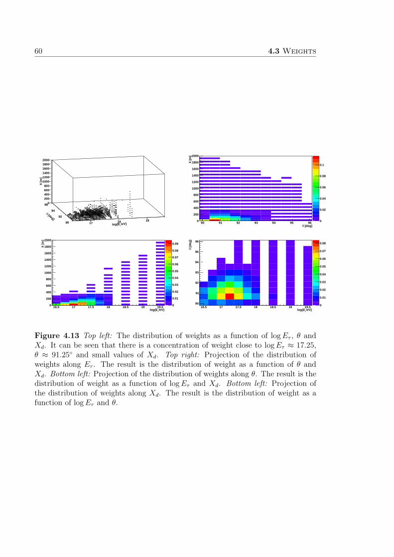
60 4.3 Weights
/eVτlogE17 18 19
[deg]
θ
90
92
94
96
X [
m]
0200400600800
100012001400160018002000
[deg]θ90 91 92 93 94 95 96
X [
m]
0
200
400
600
800
1000
1200
1400
1600
1800
2000
0
0.02
0.04
0.06
0.08
0.1
/eVτlogE16.5 17 17.5 18 18.5 19 19.5
X [
m]
0
200
400
600
800
1000
1200
1400
1600
1800
2000
0
0.01
0.02
0.03
0.04
0.05
0.06
0.07
0.08
0.09
/eVτlogE16.5 17 17.5 18 18.5 19 19.5
[d
eg]
θ
90
91
92
93
94
95
96
0
0.01
0.02
0.03
0.04
0.05
0.06
0.07
0.08
Figure 4.13 Top left: The distribution of weights as a function of logEτ , θ andXd. It can be seen that there is a concentration of weight close to logEτ ≈ 17.25,θ ≈ 91.25 and small values of Xd. Top right: Projection of the distribution ofweights along Eτ . The result is the distribution of weight as a function of θ andXd. Bottom left: Projection of the distribution of weights along θ. The result is thedistribution of weight as a function of logEτ and Xd. Bottom left: Projection ofthe distribution of weights along Xd. The result is the distribution of weight as afunction of logEτ and θ.

5Reconstruction and selectionof inclined showers
In this chapter we describe the methodology applied to select good quality events
and define a way of identifying inclined showers. Given the fact that real events
induced by UHECRs and MC simulations of nearly horizontal showers initiated
by τ leptons present singular characteristics, it was necessary to develop a set of
algorithms capable of producing good results for both neutrino MC simulations and
data samples.
The chapter is organized as follows. In Section 5.1 we present the criteria to select
quality events. In Section 5.2 we define the variables to select inclined showers and
in Section 5.3 use them to compare neutrino MC simulations to data. In Section 5.4
we summarize the quality and selection criteria.
5.1 Selection of quality events
The procedure starts with a set of events that satisfy the T3 trigger criteria
(see Sec.3.1.2) of the surface detector (SD). Within this group, real events acquired
during the periods in which the SD is working in a unstable way are discarded [117].
These are known as “Bad Periods”. Next, with the aim of obtaining a sample of
good quality events, the following sequence of procedures is applied:
1. PMT selection (Sec. 5.1.1).
2. Station selection (Sec. 5.1.2).
3. Preliminary Reconstruction (Sec. 5.1.3).
4. Additional cuts (Sec. 5.1.4).
These are explained in the following sections.
61

62 5.1 Selection of quality events
5.1.1 Photomultiplier tube selection
The neutrino search looks for extremely rare events. If a candidate appears it is
imperative to be sure that it is not the result of a malfunctioning photomultiplier
tube (PMT). We are particularly interested in PMT pathologies that induce a signal
artificially extended in time, since, as it will be shown in Chapter 6, we will use the
time spread of the signals in inclined showers to identify UHE neutrinos.
There are several reasons for tagging or discarding a PMT. We will separate
them into two groups which are explained next.
5.1.1.1 Standard cuts
This set of cuts cuts is the result of studies [118] performed with the monitoring
data (see Section3.1.2). Using this data a list of unstable PMTs is provided on
a day-to-day basis. The parameters which are studied are the anode and dynode
baselines and the dynode/anode ratio.
In the case of the baseline, it is required that their fluctuations should be small,
placing a cut on their RMS. The dynode/anode ratio is also requested to have
small fluctiantion but, more importantly, even if it is stable there are limits on its
maximum and minimum values.
In Figure 5.1 we show an example of the importance of applying these cuts before
the selection of neutrino candidates. PMTs 2 and 3 have a saturated anode signal so
the signal of the dynode is used1. The signal of the dynode in PMT 3 is very different
from PMTs 1 and 2. This PMT is disregarded in the analysis because of having a
very low dynode/anode ratio. As it will be explained in Chapter 6, neutrinos will
be selected by broad signals in time induced in the SD stations. Given that mal-
functioning PMT such as the one rejected could induce a fake neutrino candidate
this cut is of great importance.
5.1.1.2 Special cuts
When performing studies using not only the integrated charge of the FADC
traces, but also their shape, other kind of pathologies in some PMTs become appar-
ent. Most of the times they are the result of an excess of signal in the PMT trace
after the signal induced by the shower.
The method to identify this kind of pathology is described next. For each tank,
and for each dynode trace, we add up the content of bins 350 to 700. We substract
from this sum (Σi, where i stands for each PMT) the content of the maximum bin,
as well as the bin before and the bin after, to eliminate potential peaks that may be
produced by accidental single muons. Then we select stations that verify:
1A signal is saturated when in one bin the FADC channel is higher than 1024.
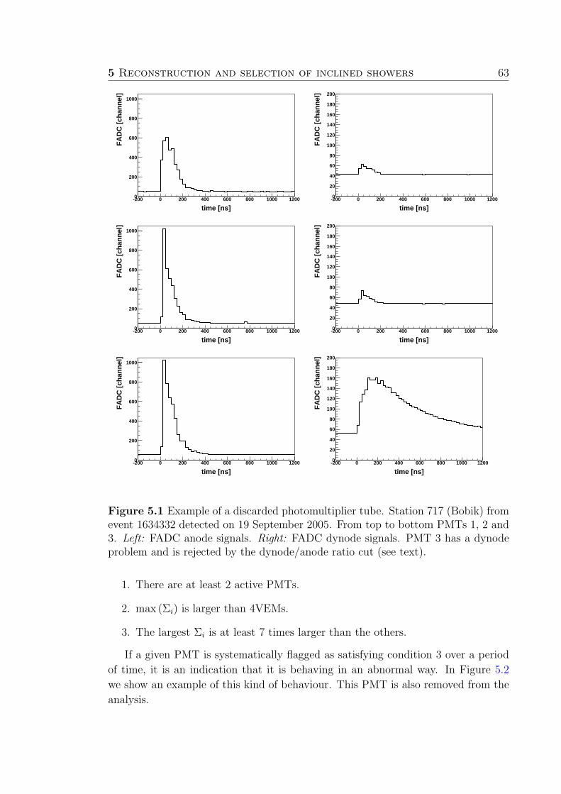
5 Reconstruction and selection of inclined showers 63
time [ns]-200 0 200 400 600 800 1000 1200
FA
DC
[ch
ann
el]
0
200
400
600
800
1000
time [ns]-200 0 200 400 600 800 1000 1200
FA
DC
[ch
ann
el]
0
20
40
60
80
100
120
140
160
180
200
time [ns]-200 0 200 400 600 800 1000 1200
FA
DC
[ch
ann
el]
0
200
400
600
800
1000
time [ns]-200 0 200 400 600 800 1000 1200
FA
DC
[ch
ann
el]
0
20
40
60
80
100
120
140
160
180
200
time [ns]-200 0 200 400 600 800 1000 1200
FA
DC
[ch
ann
el]
0
200
400
600
800
1000
time [ns]-200 0 200 400 600 800 1000 1200
FA
DC
[ch
ann
el]
0
20
40
60
80
100
120
140
160
180
200
Figure 5.1 Example of a discarded photomultiplier tube. Station 717 (Bobik) fromevent 1634332 detected on 19 September 2005. From top to bottom PMTs 1, 2 and3. Left: FADC anode signals. Right: FADC dynode signals. PMT 3 has a dynodeproblem and is rejected by the dynode/anode ratio cut (see text).
1. There are at least 2 active PMTs.
2. max (Σi) is larger than 4VEMs.
3. The largest Σi is at least 7 times larger than the others.
If a given PMT is systematically flagged as satisfying condition 3 over a period
of time, it is an indication that it is behaving in an abnormal way. In Figure 5.2
we show an example of this kind of behaviour. This PMT is also removed from the
analysis.
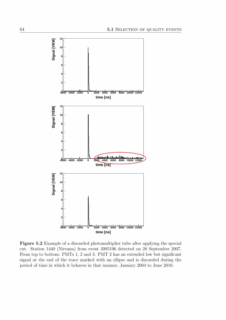
64 5.1 Selection of quality events
time [ns]-6000 -4000 -2000 0 2000 4000 6000 8000 10000 12000
Sig
nal
[V
EM
]
0
2
4
6
8
10
12
time [ns]-6000 -4000 -2000 0 2000 4000 6000 8000 10000 12000
Sig
nal
[V
EM
]
0
2
4
6
8
10
12
Figure 5.2 Example of a discarded photomultiplier tube after applying the specialcut. Station 1440 (Nirvana) from event 3995196 detected on 28 September 2007.From top to bottom: PMTs 1, 2 and 3. PMT 2 has an extended low but significantsignal at the end of the trace marked with an ellipse and is discarded during theperiod of time in which it behaves in that manner, January 2004 to June 2010.
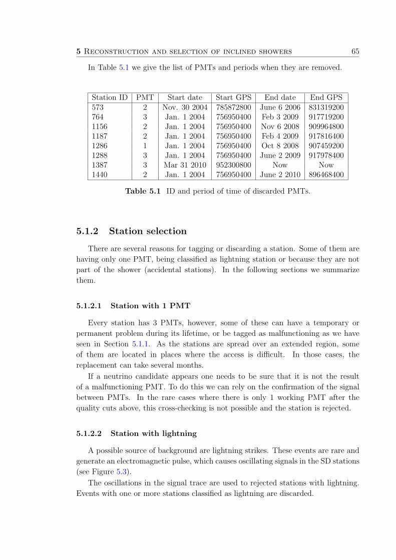
5 Reconstruction and selection of inclined showers 65
In Table 5.1 we give the list of PMTs and periods when they are removed.
Station ID PMT Start date Start GPS End date End GPS573 2 Nov. 30 2004 785872800 June 6 2006 831319200764 3 Jan. 1 2004 756950400 Feb 3 2009 9177192001156 2 Jan. 1 2004 756950400 Nov 6 2008 9099648001187 2 Jan. 1 2004 756950400 Feb 4 2009 9178164001286 1 Jan. 1 2004 756950400 Oct 8 2008 9074592001288 3 Jan. 1 2004 756950400 June 2 2009 9179784001387 3 Mar 31 2010 952300800 Now Now1440 2 Jan. 1 2004 756950400 June 2 2010 896468400
Table 5.1 ID and period of time of discarded PMTs.
5.1.2 Station selection
There are several reasons for tagging or discarding a station. Some of them are
having only one PMT, being classified as lightning station or because they are not
part of the shower (accidental stations). In the following sections we summarize
them.
5.1.2.1 Station with 1 PMT
Every station has 3 PMTs, however, some of these can have a temporary or
permanent problem during its lifetime, or be tagged as malfunctioning as we have
seen in Section 5.1.1. As the stations are spread over an extended region, some
of them are located in places where the access is difficult. In those cases, the
replacement can take several months.
If a neutrino candidate appears one needs to be sure that it is not the result
of a malfunctioning PMT. To do this we can rely on the confirmation of the signal
between PMTs. In the rare cases where there is only 1 working PMT after the
quality cuts above, this cross-checking is not possible and the station is rejected.
5.1.2.2 Station with lightning
A possible source of background are lightning strikes. These events are rare and
generate an electromagnetic pulse, which causes oscillating signals in the SD stations
(see Figure 5.3).
The oscillations in the signal trace are used to rejected stations with lightning.
Events with one or more stations classified as lightning are discarded.

66 5.1 Selection of quality events
0.3
0.2
0.1
0
-0.1
-0.2
-500 0 500 1000 1500 2000 2500 3000
Sign
al [V
EM]
Time [ns]
Figure 5.3 Example of a signal generated by lightning. This signal corresponds toevent 3995197 (January 26 2005), station 506 and PMT 3.
5.1.2.3 Accidental stations: effects of muon background
The SD is exposed to low energy cosmic radiation much more abundant than the
showers produced by UHECR. At the level of the detector (1400 meters above sea
level), the radiation is fundamentally composed by low energy atmospheric muons
with energies in the 1-10 GeV range. [119]. These particles, which are not part of
a shower, can affect the reconstruction basically in two ways:
1. Produce a T2 trigger in a station which is not part of the event: the
additional T2 trigger time will have a uniform distribution within the 50 µsec
window of the T3 trigger. As the inclined selection procedure is based on
the position and timing of the triggered stations, the extra station can result
in an incorrect estimation of the geometry of the shower. This effect can be
particularly important for low multiplicity events. We will see in Section 5.1.3
how these stations are removed.
2. Add a spurious signal to one of the stations belonging to the event:
if the accidental signal ocurrs only a few µsec before or after the particles of
the shower reach the stations, the result is that both signals are merged into
the same trace. If the first spurious signal comes firts it fixes the T2 trigger
time (see Fig. 5.4) and affects the reconstruction of the event. Even if the
spurious signal comes after and does not affect the trigger, it modifies many of
the trace observables, such as the AoP, risetime or falltime (see Section 6.2).
In order to minimize the impact of spurious signals produced by accidental low
energy muons in stations belonging to the event, the following procedure is applied.
Trace Cleaning Algorithm:
The purpose of the algorithm is the identification and removal of fractions of the
trace produced by accidental muons.

5 Reconstruction and selection of inclined showers 67
0 2000 4000 6000 8000 100000
0.2
0.4
0.6
0.8
1
1.2
1.4
1.6
1.8
Event: 6190344 - Station: 1391
Time [ns]
Sign
al [V
EM]
accidentalmuon
signal from the shower
Figure 5.4 Effect of an accidental muon in the determination of the trigger timeof the station.
The idea of the method is simple: the amount of energy provided by a muon is,
to first order, proportional to its path length in the water inside the station. Given
that the SD stations are much wider than taller (1.2 m height vs. 3.6 m diameter),
inclined muons produce in average a higher signal than the vertical ones.
Accidental muons are mostly vertical (see Fig. 5.5), so they tend to leave smaller
signals than the ones produced by inclined showers. This fact can be exploited to
identify fractions of the trace produced by atmospheric muons.
(E/GeV)10
log-1 0 1 2 3 4 50
0.1
0.2
0.3
0.4
0.5
0.6
0.7
0.8
0.9
1
0
0.001
0.002
0.003
0.004
0.005
]-1 s
-2cm
-1sr
-1[G
eVse
cμΦ
cos
θ
.
Figure 5.5 Atmospheric muonic flux according to a parametrization given in [119,120]. It can be observed that roughly ∼ 95% of the total flux arrives at θ > 50
(cos θ > 0.6).
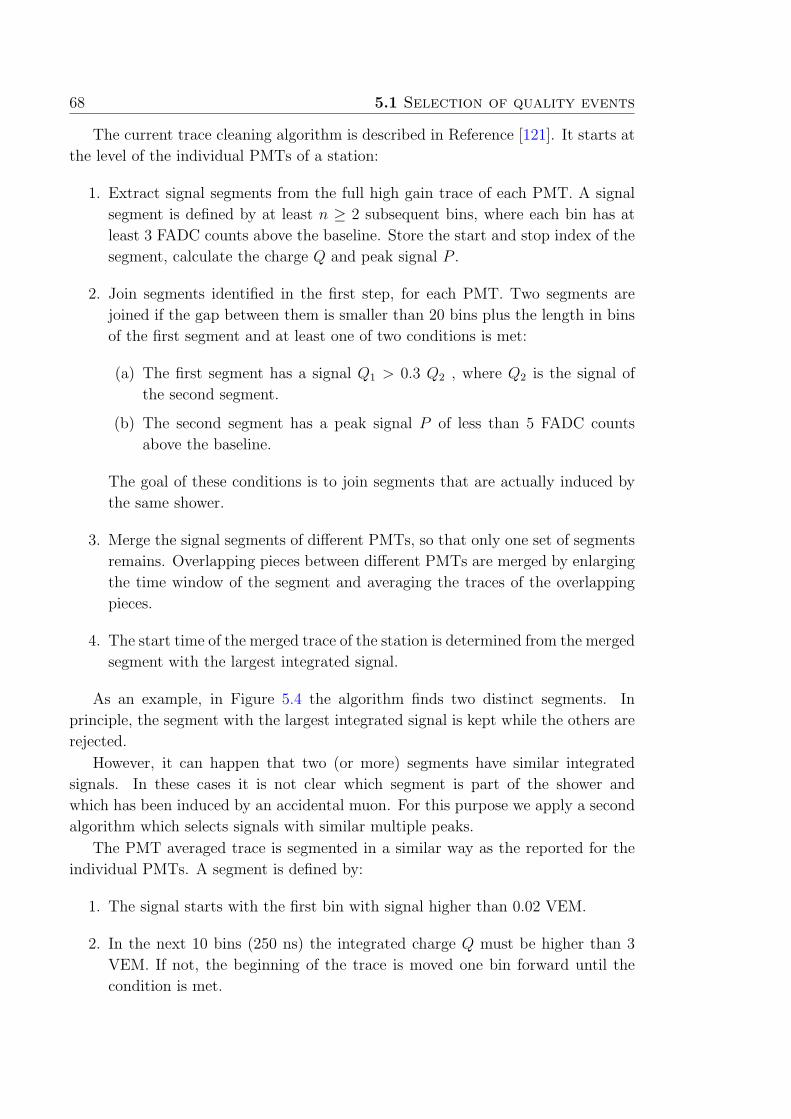
68 5.1 Selection of quality events
The current trace cleaning algorithm is described in Reference [121]. It starts at
the level of the individual PMTs of a station:
1. Extract signal segments from the full high gain trace of each PMT. A signal
segment is defined by at least n ≥ 2 subsequent bins, where each bin has at
least 3 FADC counts above the baseline. Store the start and stop index of the
segment, calculate the charge Q and peak signal P .
2. Join segments identified in the first step, for each PMT. Two segments are
joined if the gap between them is smaller than 20 bins plus the length in bins
of the first segment and at least one of two conditions is met:
(a) The first segment has a signal Q1 > 0.3 Q2 , where Q2 is the signal of
the second segment.
(b) The second segment has a peak signal P of less than 5 FADC counts
above the baseline.
The goal of these conditions is to join segments that are actually induced by
the same shower.
3. Merge the signal segments of different PMTs, so that only one set of segments
remains. Overlapping pieces between different PMTs are merged by enlarging
the time window of the segment and averaging the traces of the overlapping
pieces.
4. The start time of the merged trace of the station is determined from the merged
segment with the largest integrated signal.
As an example, in Figure 5.4 the algorithm finds two distinct segments. In
principle, the segment with the largest integrated signal is kept while the others are
rejected.
However, it can happen that two (or more) segments have similar integrated
signals. In these cases it is not clear which segment is part of the shower and
which has been induced by an accidental muon. For this purpose we apply a second
algorithm which selects signals with similar multiple peaks.
The PMT averaged trace is segmented in a similar way as the reported for the
individual PMTs. A segment is defined by:
1. The signal starts with the first bin with signal higher than 0.02 VEM.
2. In the next 10 bins (250 ns) the integrated charge Q must be higher than 3
VEM. If not, the beginning of the trace is moved one bin forward until the
condition is met.

5 Reconstruction and selection of inclined showers 69
3. The end of the signal is defined when the next 15 bins all have a signal lower
than 0.02 VEM/bin.
4. Two relevant parameters calculated over the segment are:
(a) nBoT : number of bins with signal higher than 0.02 VEM.
(b) QT : sum of the signal over the bins with signal higher than 0.02 VEM.
Every segment has a score defined by s = nBoT × QT . The segments induced by
atmospheric muons tend to have small values of s compared to the ones with larger
values of s, either because they are induced by inclined muons (more intense) or by
the electromagnetic component (more extended in time). If there are more than one
segment fullfilling that s > 0.15 smax, with smax the maximum score, the station is
rejected because it cannot be unambiguously decided which of the segments is due
to an accidental muon. If not, all segments except the one with smax are rejected,
and the station is kept.
In Figure 5.6 we show an example of a station presenting 3 similar segments. A
station like this is removed from the event before applying the inclined reconstruc-
tion.
Event: 1702869 - Station: 825
Time [nsec]
Sign
al [V
EM]
Figure 5.6 Trace presenting multiple signal segments with similar characteristicsin which it is not possible to determine the trigger time. The numbers next to eachsegment indicate the score s assigned to every segment according to the proceduredescribed in the text.
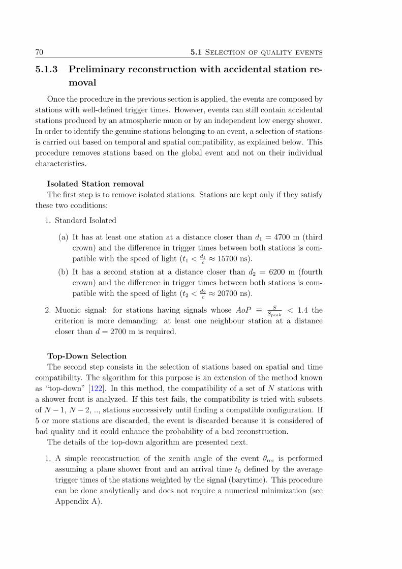
70 5.1 Selection of quality events
5.1.3 Preliminary reconstruction with accidental station re-
moval
Once the procedure in the previous section is applied, the events are composed by
stations with well-defined trigger times. However, events can still contain accidental
stations produced by an atmospheric muon or by an independent low energy shower.
In order to identify the genuine stations belonging to an event, a selection of stations
is carried out based on temporal and spatial compatibility, as explained below. This
procedure removes stations based on the global event and not on their individual
characteristics.
Isolated Station removal
The first step is to remove isolated stations. Stations are kept only if they satisfy
these two conditions:
1. Standard Isolated
(a) It has at least one station at a distance closer than d1 = 4700 m (third
crown) and the difference in trigger times between both stations is com-
patible with the speed of light (t1 <d1c≈ 15700 ns).
(b) It has a second station at a distance closer than d2 = 6200 m (fourth
crown) and the difference in trigger times between both stations is com-
patible with the speed of light (t2 <d2c≈ 20700 ns).
2. Muonic signal: for stations having signals whose AoP ≡ SSpeak
< 1.4 the
criterion is more demanding: at least one neighbour station at a distance
closer than d = 2700 m is required.
Top-Down Selection
The second step consists in the selection of stations based on spatial and time
compatibility. The algorithm for this purpose is an extension of the method known
as “top-down” [122]. In this method, the compatibility of a set of N stations with
a shower front is analyzed. If this test fails, the compatibility is tried with subsets
of N − 1, N − 2, .., stations successively until finding a compatible configuration. If
5 or more stations are discarded, the event is discarded because it is considered of
bad quality and it could enhance the probability of a bad reconstruction.
The details of the top-down algorithm are presented next.
1. A simple reconstruction of the zenith angle of the event θrec is performed
assuming a plane shower front and an arrival time t0 defined by the average
trigger times of the stations weighted by the signal (barytime). This procedure
can be done analytically and does not require a numerical minimization (see
Appendix A).
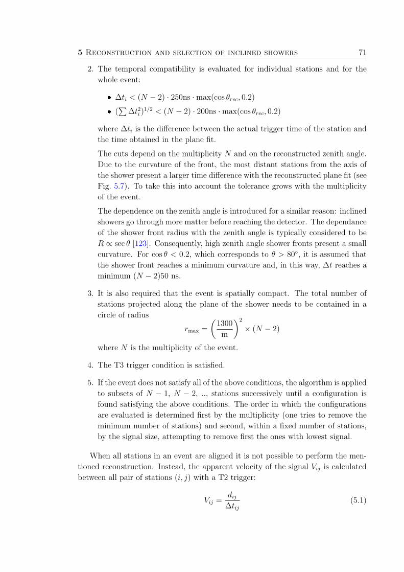
5 Reconstruction and selection of inclined showers 71
2. The temporal compatibility is evaluated for individual stations and for the
whole event:
❼ ∆ti < (N − 2) · 250ns ·max(cos θrec, 0.2)
❼ (∑
∆t2i )1/2 < (N − 2) · 200ns ·max(cos θrec, 0.2)
where ∆ti is the difference between the actual trigger time of the station and
the time obtained in the plane fit.
The cuts depend on the multiplicity N and on the reconstructed zenith angle.
Due to the curvature of the front, the most distant stations from the axis of
the shower present a larger time difference with the reconstructed plane fit (see
Fig. 5.7). To take this into account the tolerance grows with the multiplicity
of the event.
The dependence on the zenith angle is introduced for a similar reason: inclined
showers go through more matter before reaching the detector. The dependance
of the shower front radius with the zenith angle is typically considered to be
R ∝ sec θ [123]. Consequently, high zenith angle shower fronts present a small
curvature. For cos θ < 0.2, which corresponds to θ > 80, it is assumed that
the shower front reaches a minimum curvature and, in this way, ∆t reaches a
minimum (N − 2)50 ns.
3. It is also required that the event is spatially compact. The total number of
stations projected along the plane of the shower needs to be contained in a
circle of radius
rmax =
(1300
m
)2
× (N − 2)
where N is the multiplicity of the event.
4. The T3 trigger condition is satisfied.
5. If the event does not satisfy all of the above conditions, the algorithm is applied
to subsets of N − 1, N − 2, .., stations successively until a configuration is
found satisfying the above conditions. The order in which the configurations
are evaluated is determined first by the multiplicity (one tries to remove the
minimum number of stations) and second, within a fixed number of stations,
by the signal size, attempting to remove first the ones with lowest signal.
When all stations in an event are aligned it is not possible to perform the men-
tioned reconstruction. Instead, the apparent velocity of the signal Vij is calculated
between all pair of stations (i, j) with a T2 trigger:
Vij =dij∆tij
(5.1)
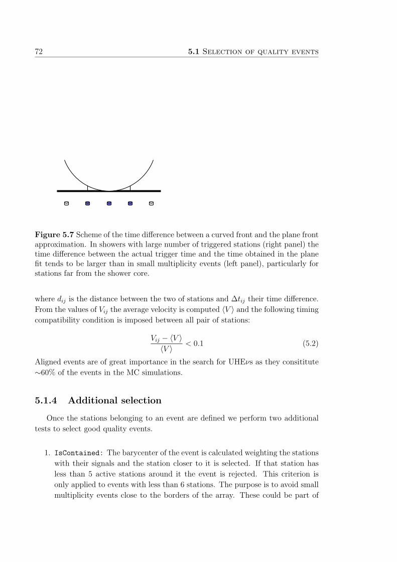
72 5.1 Selection of quality events
Δt
Shower generating a low multiplicity event
Δt
Shower generating a high multiplicity event
Figure 5.7 Scheme of the time difference between a curved front and the plane frontapproximation. In showers with large number of triggered stations (right panel) thetime difference between the actual trigger time and the time obtained in the planefit tends to be larger than in small multiplicity events (left panel), particularly forstations far from the shower core.
where dij is the distance between the two of stations and ∆tij their time difference.
From the values of Vij the average velocity is computed 〈V 〉 and the following timing
compatibility condition is imposed between all pair of stations:
Vij − 〈V 〉〈V 〉 < 0.1 (5.2)
Aligned events are of great importance in the search for UHEνs as they consititute
∼60% of the events in the MC simulations.
5.1.4 Additional selection
Once the stations belonging to an event are defined we perform two additional
tests to select good quality events.
1. IsContained: The barycenter of the event is calculated weighting the stations
with their signals and the station closer to it is selected. If that station has
less than 5 active stations around it the event is rejected. This criterion is
only applied to events with less than 6 stations. The purpose is to avoid small
multiplicity events close to the borders of the array. These could be part of

5 Reconstruction and selection of inclined showers 73
a higher multiplicity event where the core fell outside the array, and hence a
large fraction of the event is missing.
2. hottestHasNeighbour: It is required that the station with the highest signal
has at least one station with signal in the surrounding crown of stations. If
the condition is not met the event is rejected.
5.2 Variables for selection of inclined showers
In this section we define the two variables used to select inclined events: the
length over width of the footprint, L/W , and the velocity at ground, 〈V 〉.
5.2.1 Event footprint
The pattern of stations with signal in inclined events produces elongated foot-
prints on the SD. This property can be characterized by constructing a “signal
moment tensor”:
S =∑
i
si, 〈X〉 =∑
i
sixi/S, 〈Y 〉 =∑
i
siyi/S
Ixx =∑
i
si(xi − 〈X〉)2/S, Iyy =∑
i
si(yi − 〈Y 〉)2/S
Ixy = Iyx =∑
i
si(xi − 〈X〉)(yi − 〈Y 〉)/S (5.3)
This object describes the spatial distribution of signal in the same way as the inertia
tensor does with the mass. Following the analogy (see Fig. 5.8)2 one can obtain the
size of the principal axis of the elliptically-shaped footprint as:
L2 =Ixx + Iyy +
√
(Ixx − Iyy)2 + I2xy
2
W 2 =Ixx + Iyy −
√
(Ixx − Iyy)2 + I2xy
2(5.4)
where L (Length) and W (Width) correspond respectively to the size of the major
and minor axes.
It is possible that a vertical shower together with an accidental station gives
a 〈V 〉 consistent with an inclined shower. However, these events don’t have an
elongated footprint. In this way, the ratio L/W can be used as a quality criterion
to select inclined events.
2To calculate the ellipse, W and L we use all T1 stations.

74 5.3 Performance of the inclined shower selection
major axis
minor axis
Direction of the major axis from the obteined ellipse
Lij
ΔTij
Figure 5.8 Left: Sketch of the elliptically-shaped footprint of the shower thatrepresents the spatial configuration of an inclined event. Right: Sketch showingthe calculation of the apparent signal speed Vij between stations i and j.
5.2.2 Ground speed
In an inclined event, the axis of the shower is almost parallel to the direction of
the major axis of the ellipse. In this way the signal speed at the ground (V ) along
this direction gives a good approximation to the zenith angle.
sin θ ≃ 〈V 〉c
(5.5)
In order to estimate 〈V 〉 for an event, one averages the pairs of velocities Vij ≡Lij/∆Tij between stations whose relative distance, projected along the major axis,
Lij, is larger than 1000 m (see right panel of Fig. 5.8)3. One does not consider pairs
of stations with distances Lij < 1000 m to avoid Vij values with large uncertainty
due to the fluctuations in the trigger time of the stations.
5.3 Performance of the inclined shower selection
In this section we compare the ν MC sample with the data sample. The purpose
is to analize the variables described in the previous Section for both samples. Then
we define the selection cuts and, finally, we evaluate the performance and efficiency
of the inclined shower selection. The procedure will treat 3 stations events separately
from the rest.
For reference, the sum of weights, defined in Section 4.3, for events with 4 stations
or more, amounts to ∼ 70%, while events with 3 stations account for ∼ 30%.
3To calculate the ground speed velocity we use only T2 stations.

5 Reconstruction and selection of inclined showers 75
5.3.1 Events with 4 stations or more
The inclined selection criteria for events with 4 stations or more are:
❼LW
> 5
❼ 0.29 mns
< 〈V 〉 < 0.31 mns
❼ RMS(V ) < 0.08 mns
In Figures 5.9, 5.10 and 5.11 we respectively show the distributions of W/L, 〈V 〉and RMS(V ) for data from 1 January 2004 up to 31 October 2007 as well as for
the simulated neutrino events. We also show the values of the cuts and the region
selected. The plots illustrate that the Inclined Shower Selection above keeps most
of the MC events.
Figure 5.9 Distribution of W/L in data and in MC simulations of ES ντ -inducedevents. The vertical dotted line corresponds to the cut applied in the InclinedSelection at W/L < 0.2 (or equivalently L/W > 5). We have applied a relaxed cuton 〈V 〉 < 0.35m
ns. Notice that we have plotted W/L instead of L/W because aligned
events have an infinite value of L/W (zero value of W/L).
5.3.2 Events with 3 stations
The sum of the weights, defined in Section 4.3, for 3-station events is ∼30%.
This non-negligible contribution to the expected yield makes it important to design
a criterion to efficiently select these events.
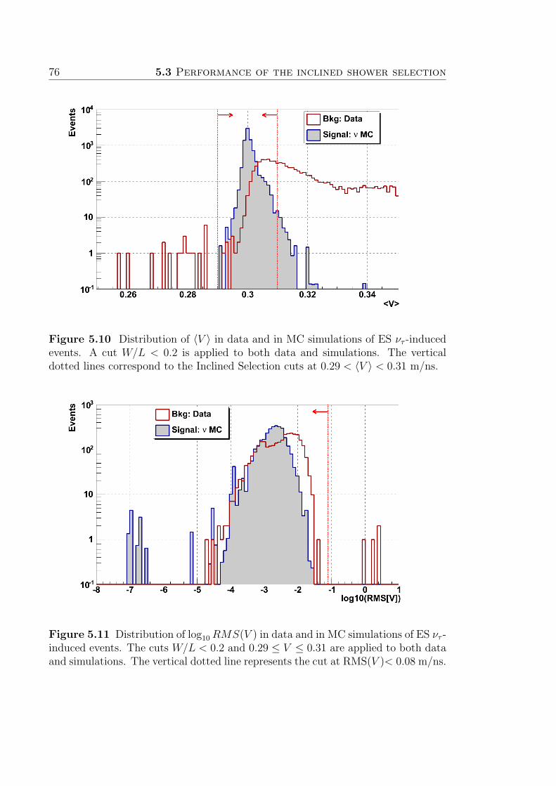
76 5.3 Performance of the inclined shower selection
Figure 5.10 Distribution of 〈V 〉 in data and in MC simulations of ES ντ -inducedevents. A cut W/L < 0.2 is applied to both data and simulations. The verticaldotted lines correspond to the Inclined Selection cuts at 0.29 < 〈V 〉 < 0.31 m/ns.
Figure 5.11 Distribution of log10 RMS(V ) in data and in MC simulations of ES ντ -induced events. The cuts W/L < 0.2 and 0.29 ≤ V ≤ 0.31 are applied to both dataand simulations. The vertical dotted line represents the cut at RMS(V )< 0.08 m/ns.

5 Reconstruction and selection of inclined showers 77
The number of possible 3-station configurations that can satisfy the geometrical
requirement of a T3 trigger is only 7. In Fig. 5.12 we show a sketch of these 7
configurations. In this Section we study the effects of replacing the cut on L/W for
3-station events with a selection of only certain configurations among the 7 possible
ones. Ideally, one would like to keep those configurations that contribute most to
the total yield but at the same time to eliminate those that are prone to induce fake
neutrino candidates in data.
Figure 5.12 Sketches of the 7 possible T3 configurations for 3-station events.Full circles indicate the triggered stations. Top: From left to right: configurationsnumber 1 to 3. Bottom: From left to right: configurations number 4 to 7.
In Table 5.2 we show the frequency of appearance in the MC neutrino sample at
trigger level, of the configurations shown in Fig. 5.12. At trigger level the dominant
configurations turn out to be numbers 1 and 5.
After applying the quality selection criteria defined in Section 5.1 the number
of events belonging to each one of the 3-station configurations can change mainly
for two reasons. Firstly, there are 3-station events that do not pass the criteria.
Secondly, events with more than 3 stations can lose some of them and become 3-
station events. Note, in fact, that the number od 3-station events increases after
applying the quality ctus. In Table 5.3 we show the frequency of appearance of the
configurations in Fig. 5.12 after the quality selection criteria are applied.
Tables 5.2 and 5.3 show similar results. In both cases, the two dominant con-
figurations are numbers 1 and 5. The reasons why the other configurations do not
appear in simulations as frequently as these are:
❼ Configurations 2 and 3 are too compact and wide. ES neutrinos typically
have very elongated footprints so if the event is wide enough to trigger these
stations, it will most probably trigger also more stations along the direction
of the shower.
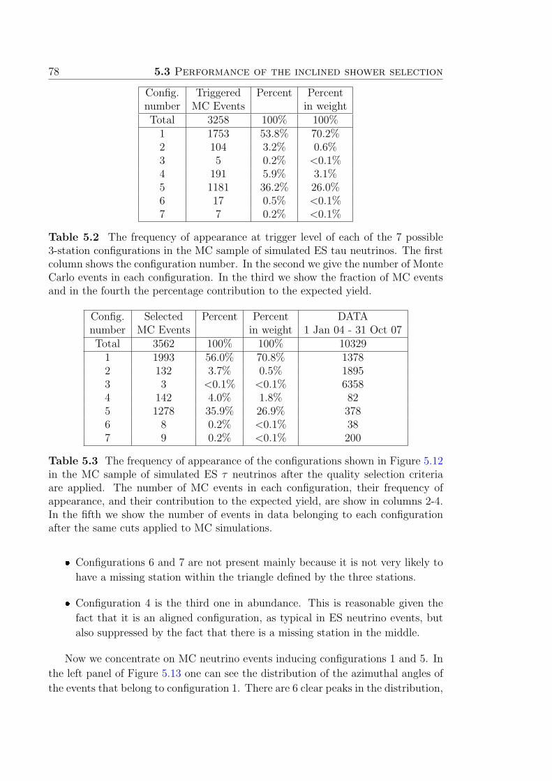
78 5.3 Performance of the inclined shower selection
Config. Triggered Percent Percentnumber MC Events in weightTotal 3258 100% 100%1 1753 53.8% 70.2%2 104 3.2% 0.6%3 5 0.2% <0.1%4 191 5.9% 3.1%5 1181 36.2% 26.0%6 17 0.5% <0.1%7 7 0.2% <0.1%
Table 5.2 The frequency of appearance at trigger level of each of the 7 possible3-station configurations in the MC sample of simulated ES tau neutrinos. The firstcolumn shows the configuration number. In the second we give the number of MonteCarlo events in each configuration. In the third we show the fraction of MC eventsand in the fourth the percentage contribution to the expected yield.
Config. Selected Percent Percent DATAnumber MC Events in weight 1 Jan 04 - 31 Oct 07Total 3562 100% 100% 103291 1993 56.0% 70.8% 13782 132 3.7% 0.5% 18953 3 <0.1% <0.1% 63584 142 4.0% 1.8% 825 1278 35.9% 26.9% 3786 8 0.2% <0.1% 387 9 0.2% <0.1% 200
Table 5.3 The frequency of appearance of the configurations shown in Figure 5.12in the MC sample of simulated ES τ neutrinos after the quality selection criteriaare applied. The number of MC events in each configuration, their frequency ofappearance, and their contribution to the expected yield, are show in columns 2-4.In the fifth we show the number of events in data belonging to each configurationafter the same cuts applied to MC simulations.
❼ Configurations 6 and 7 are not present mainly because it is not very likely to
have a missing station within the triangle defined by the three stations.
❼ Configuration 4 is the third one in abundance. This is reasonable given the
fact that it is an aligned configuration, as typical in ES neutrino events, but
also suppressed by the fact that there is a missing station in the middle.
Now we concentrate on MC neutrino events inducing configurations 1 and 5. In
the left panel of Figure 5.13 one can see the distribution of the azimuthal angles of
the events that belong to configuration 1. There are 6 clear peaks in the distribution,
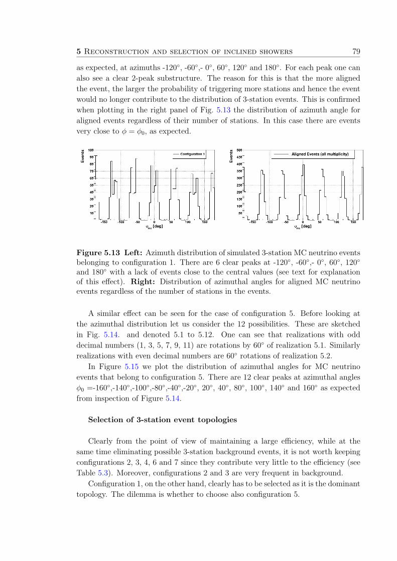
5 Reconstruction and selection of inclined showers 79
as expected, at azimuths -120, -60,- 0, 60, 120 and 180. For each peak one can
also see a clear 2-peak substructure. The reason for this is that the more aligned
the event, the larger the probability of triggering more stations and hence the event
would no longer contribute to the distribution of 3-station events. This is confirmed
when plotting in the right panel of Fig. 5.13 the distribution of azimuth angle for
aligned events regardless of their number of stations. In this case there are events
very close to φ = φ0, as expected.
Figure 5.13 Left: Azimuth distribution of simulated 3-station MC neutrino eventsbelonging to configuration 1. There are 6 clear peaks at -120, -60,- 0, 60, 120
and 180 with a lack of events close to the central values (see text for explanationof this effect). Right: Distribution of azimuthal angles for aligned MC neutrinoevents regardless of the number of stations in the events.
A similar effect can be seen for the case of configuration 5. Before looking at
the azimuthal distribution let us consider the 12 possibilities. These are sketched
in Fig. 5.14. and denoted 5.1 to 5.12. One can see that realizations with odd
decimal numbers (1, 3, 5, 7, 9, 11) are rotations by 60 of realization 5.1. Similarly
realizations with even decimal numbers are 60 rotations of realization 5.2.
In Figure 5.15 we plot the distribution of azimuthal angles for MC neutrino
events that belong to configuration 5. There are 12 clear peaks at azimuthal angles
φ0 =-160,-140,-100,-80,-40,-20, 20, 40, 80, 100, 140 and 160 as expected
from inspection of Figure 5.14.
Selection of 3-station event topologies
Clearly from the point of view of maintaining a large efficiency, while at the
same time eliminating possible 3-station background events, it is not worth keeping
configurations 2, 3, 4, 6 and 7 since they contribute very little to the efficiency (see
Table 5.3). Moreover, configurations 2 and 3 are very frequent in background.
Configuration 1, on the other hand, clearly has to be selected as it is the dominant
topology. The dilemma is whether to choose also configuration 5.
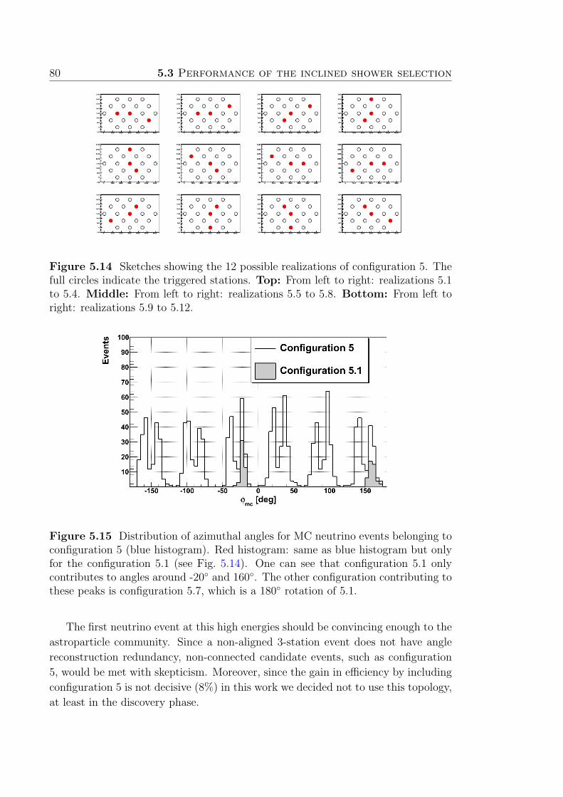
80 5.3 Performance of the inclined shower selection
Figure 5.14 Sketches showing the 12 possible realizations of configuration 5. Thefull circles indicate the triggered stations. Top: From left to right: realizations 5.1to 5.4. Middle: From left to right: realizations 5.5 to 5.8. Bottom: From left toright: realizations 5.9 to 5.12.
Figure 5.15 Distribution of azimuthal angles for MC neutrino events belonging toconfiguration 5 (blue histogram). Red histogram: same as blue histogram but onlyfor the configuration 5.1 (see Fig. 5.14). One can see that configuration 5.1 onlycontributes to angles around -20 and 160. The other configuration contributing tothese peaks is configuration 5.7, which is a 180 rotation of 5.1.
The first neutrino event at this high energies should be convincing enough to the
astroparticle community. Since a non-aligned 3-station event does not have angle
reconstruction redundancy, non-connected candidate events, such as configuration
5, would be met with skepticism. Moreover, since the gain in efficiency by including
configuration 5 is not decisive (8%) in this work we decided not to use this topology,
at least in the discovery phase.
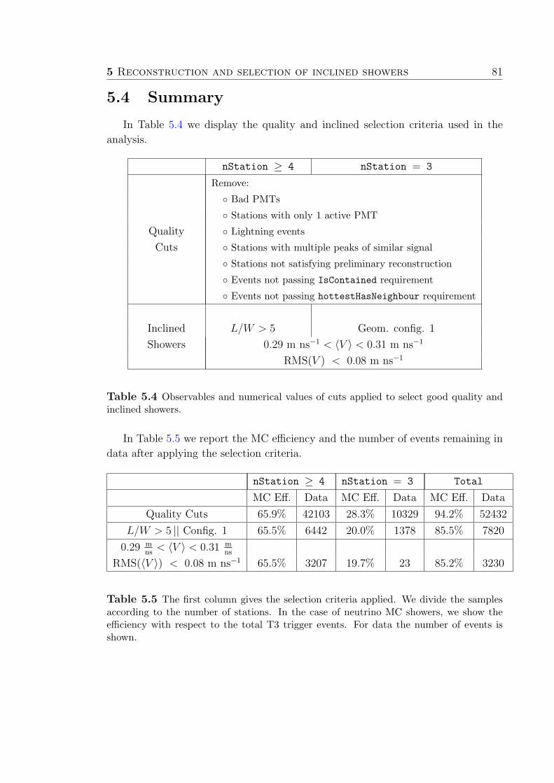
5 Reconstruction and selection of inclined showers 81
5.4 Summary
In Table 5.4 we display the quality and inclined selection criteria used in the
analysis.
nStation ≥ 4 nStation = 3
Remove:
Bad PMTs
Stations with only 1 active PMT
Quality Lightning events
Cuts Stations with multiple peaks of similar signal
Stations not satisfying preliminary reconstruction
Events not passing IsContained requirement
Events not passing hottestHasNeighbour requirement
Inclined L/W > 5 Geom. config. 1
Showers 0.29 m ns−1 < 〈V 〉 < 0.31 m ns−1
RMS(V ) < 0.08 m ns−1
Table 5.4 Observables and numerical values of cuts applied to select good quality andinclined showers.
In Table 5.5 we report the MC efficiency and the number of events remaining in
data after applying the selection criteria.
nStation ≥ 4 nStation = 3 Total
MC Eff. Data MC Eff. Data MC Eff. Data
Quality Cuts 65.9% 42103 28.3% 10329 94.2% 52432
L/W > 5 || Config. 1 65.5% 6442 20.0% 1378 85.5% 7820
0.29 mns
< 〈V 〉 < 0.31 mns
RMS(〈V 〉) < 0.08 m ns−1 65.5% 3207 19.7% 23 85.2% 3230
Table 5.5 The first column gives the selection criteria applied. We divide the samplesaccording to the number of stations. In the case of neutrino MC showers, we show theefficiency with respect to the total T3 trigger events. For data the number of events isshown.

6Neutrino identification
In the previous chapter we have discussed the selection of good quality inclined
showers. In this chapter we analyze the identification of showers generated by τ
leptons emerging from the Earth in the presence of the dominant background of
hadronic showers.
In order to avoid biases in the analysis, this work adopted a “blind search”
scheme. Roodman [124] defines a blind search as one whose methodology and tools
are developed before performing the measurement. Within this framework the anal-
ysis reduces the possible biases coming from the prejudices a researcher may have
due to theoretical reasons or results from previous experiments.
The development of identification algorithms requires the knowledge of the fea-
tures that distinguish signal from background showers. Since until now no neutrinos
have been found, we have to rely on MC simulations to characterize signal events.
For background, on the other hand, we have the choice of using actual data or
a simulation of hadronic showers. There are several reasons to choose the former.
In the first place, since the cosmic ray spectrum falls as E−3, the background will
be mainly composed of hadronic showers at the lowest energies than trigger the
array. The trigger efficiency itself decreases at low energies, with εtrig < 1% at
energies below 1018.5 eV and zenith angles higher than 80. The simulation of the
background would thus require the generation of more than 100 events for each
shower accepted in the final sample. In the second place, even if the generation of
such a huge number of showers were feasible, the hadronic showers most likely to
be confused with neutrinos are those with extreme or abnormal behaviour of the
detector, characteristics that are most probably not included in the simulation.
The data themselves, on the other hand, are an excellent model for the back-
ground. They are overwhelmingly (if not totally) constituted by hadronic events,
83
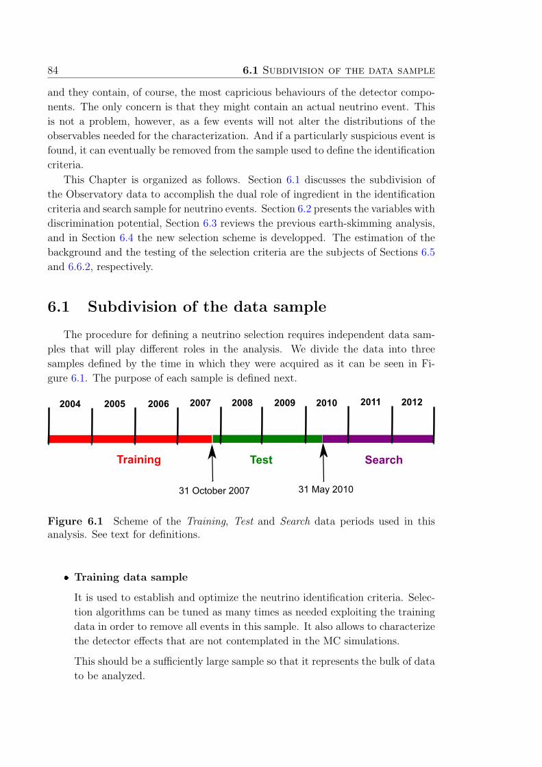
84 6.1 Subdivision of the data sample
and they contain, of course, the most capricious behaviours of the detector compo-
nents. The only concern is that they might contain an actual neutrino event. This
is not a problem, however, as a few events will not alter the distributions of the
observables needed for the characterization. And if a particularly suspicious event is
found, it can eventually be removed from the sample used to define the identification
criteria.
This Chapter is organized as follows. Section 6.1 discusses the subdivision of
the Observatory data to accomplish the dual role of ingredient in the identification
criteria and search sample for neutrino events. Section 6.2 presents the variables with
discrimination potential, Section 6.3 reviews the previous earth-skimming analysis,
and in Section 6.4 the new selection scheme is developped. The estimation of the
background and the testing of the selection criteria are the subjects of Sections 6.5
and 6.6.2, respectively.
6.1 Subdivision of the data sample
The procedure for defining a neutrino selection requires independent data sam-
ples that will play different roles in the analysis. We divide the data into three
samples defined by the time in which they were acquired as it can be seen in Fi-
gure 6.1. The purpose of each sample is defined next.
Training Test Search
2004 2005 2006 2007 2008 2009 2010 2011 2012
31 October 2007 31 May 2010
Figure 6.1 Scheme of the Training, Test and Search data periods used in thisanalysis. See text for definitions.
❼ Training data sample
It is used to establish and optimize the neutrino identification criteria. Selec-
tion algorithms can be tuned as many times as needed exploiting the training
data in order to remove all events in this sample. It also allows to characterize
the detector effects that are not contemplated in the MC simulations.
This should be a sufficiently large sample so that it represents the bulk of data
to be analyzed.
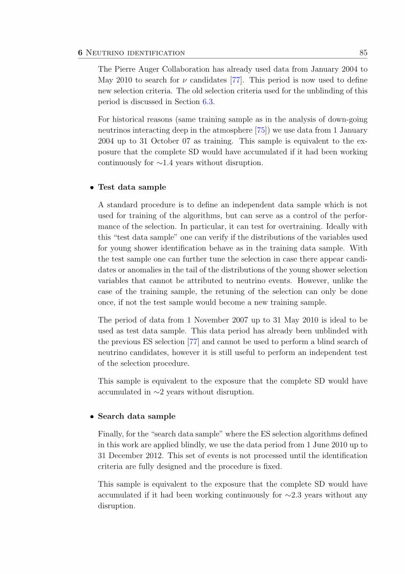
6 Neutrino identification 85
The Pierre Auger Collaboration has already used data from January 2004 to
May 2010 to search for ν candidates [77]. This period is now used to define
new selection criteria. The old selection criteria used for the unblinding of this
period is discussed in Section 6.3.
For historical reasons (same training sample as in the analysis of down-going
neutrinos interacting deep in the atmosphere [75]) we use data from 1 January
2004 up to 31 October 07 as training. This sample is equivalent to the ex-
posure that the complete SD would have accumulated if it had been working
continuously for ∼1.4 years without disruption.
❼ Test data sample
A standard procedure is to define an independent data sample which is not
used for training of the algorithms, but can serve as a control of the perfor-
mance of the selection. In particular, it can test for overtraining. Ideally with
this “test data sample” one can verify if the distributions of the variables used
for young shower identification behave as in the training data sample. With
the test sample one can further tune the selection in case there appear candi-
dates or anomalies in the tail of the distributions of the young shower selection
variables that cannot be attributed to neutrino events. However, unlike the
case of the training sample, the retuning of the selection can only be done
once, if not the test sample would become a new training sample.
The period of data from 1 November 2007 up to 31 May 2010 is ideal to be
used as test data sample. This data period has already been unblinded with
the previous ES selection [77] and cannot be used to perform a blind search of
neutrino candidates, however it is still useful to perform an independent test
of the selection procedure.
This sample is equivalent to the exposure that the complete SD would have
accumulated in ∼2 years without disruption.
❼ Search data sample
Finally, for the “search data sample” where the ES selection algorithms defined
in this work are applied blindly, we use the data period from 1 June 2010 up to
31 December 2012. This set of events is not processed until the identification
criteria are fully designed and the procedure is fixed.
This sample is equivalent to the exposure that the complete SD would have
accumulated if it had been working continuously for ∼2.3 years without any
disruption.
86 6.2 Selection: Idea and potential variables
6.2 Selection: Idea and potential variables
In Chapter 2 we discussed that inclined hadronic showers are dominated by the
muonic component while inclined neutrino induced showers present a significant
amount of electromagnetic (EM) component at the level of the surface detector
stations (young showers). In the case of DG neutrinos the EM component is con-
centrated in the region of the ground where the event hits first (the so-called early
region). On the other hand, Earth-skimming neutrinos which are expected to be
observed through the decay of an emerging τ have an EM component in all stations.
This is ilustrated on Figure 6.2 and is supported with MC simulations, as it will be
shown in Section 6.4.
muons
electrons & fotons
firstinteraction
muons
electrons & fotonsτ decay
muons
electrons & fotons
first interaction
Figure 6.2 Top: Scheme of an inclined shower initiated by a hadron which interactshigh in the atmosphere. Middle: Deep shower initiated by a DG neutrino. The earlyregion presents a significant EM component when reaching the detector. BottomShower generated by the decay of a τ emerging from the Earth. The EM componentis present along all stations.

6 Neutrino identification 87
Consequently, the idea of detecting neutrinos is to look for inclined showers
with EM component at ground. We have already defined the inclined selection in
Chapter 5 so now we proceed to select events with high electromagnetic component
within this sample.
The stations having EM component typically have signals with a duration of
the order of few hundred of nanoseconds. On the contrary, stations that are only
reached by muons exhibit signals that extend for tens of nanoseconds.
The basic idea to identify stations hit by a significant electromagnetic component
is simple. We use the trace of the FADC to construct observables correlated with
the time structure of the signal. Several variables related to the time structure of the
signal are expected to show differences between EM and muonic traces (see Fig. 3.6).
Next, we summarize some of the observables which were studied.
❼ Number of ToT station: In Section 3.1.2 we have discussed that typically
short (extended) signals have a T2 (ToT) trigger. Consequently, a very simple
idea to identify neutrinos is to count the number of ToT stations or use the
ratio between the number of T2 and ToT. The disadvantage of this variable
is that their distributions are very difficult to use when trying to estimate the
expected background.
❼ RT/FT: The risetime and falltime are defined as the time it takes a signal to
go from 10% to 50% and from 50% to 90% of the total value. They have as an
evident advantage the fact that they are directly correlated with the physical
magnitude that we want to measure (duration of the signal). Both variables
show discrimination between hadronic and neutrino showers. On the other
hand, their distributions present long non-exponential tails which make them
unsuitable for ν searches because background showers induced by UHECRs
can be missidentified as ν candidates (see Figure 6.3). Moreover, we have seen
in Section 5.1.1.2 that there are PMTs showing anomalies after a physical
signal. This anomalies would result in an overestimation of the fall time if, by
chance, the PMT is not rejected.
❼ AoP: the area divided by the peak of the signal is denoted AoP. This mag-
nitude is defined as the ratio between the integral of the FADC trace and the
maximum value (see Fig. 6.4). It is calibrated so that a vertical muon has
AoP=1. EM signals, extended over time, have higher values of AoP than the
ones produced by muon fronts, of short duration. As shown in Figure 6.5 there
is a rather good separation between the training data and the ν simulations,
and, more importantly, the distribution in data does not present very long
tails extended towards the region where the ν simulations are concentrated.
The same is true for the AoP of other stations in the events. The possibility
to missidentify an UHECR-induced shower as a ν candidate is smaller than in
the case of RT and FT. Also in Figure 6.5 we show that the variable AoP is
very correlated to FT. The same happens with RT.
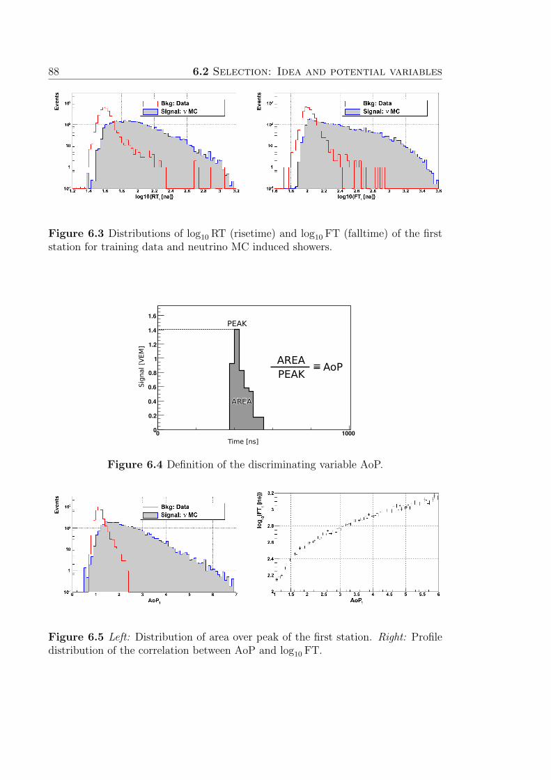
88 6.2 Selection: Idea and potential variables
Figure 6.3 Distributions of log10 RT (risetime) and log10 FT (falltime) of the firststation for training data and neutrino MC induced showers.
AREAAREA
Time [ns]
Sign
al [V
EM]
AREAPEAK AoP
PEAK
Figure 6.4 Definition of the discriminating variable AoP.
Figure 6.5 Left: Distribution of area over peak of the first station. Right: Profiledistribution of the correlation between AoP and log10 FT.
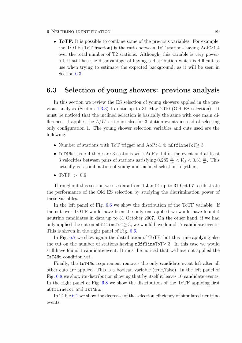
6 Neutrino identification 89
❼ ToTF: It is possible to combine some of the previous variables. For example,
the TOTF (ToT fraction) is the ratio between ToT stations having AoP≥1.4
over the total number of T2 stations. Although, this variable is very power-
ful, it still has the disadvantage of having a distribution which is difficult to
use when trying to estimate the expected background, as it will be seen in
Section 6.3.
6.3 Selection of young showers: previous analysis
In this section we review the ES selection of young showers applied in the pre-
vious analysis (Section 1.3.3) to data up to 31 May 2010 (Old ES selection). It
must be noticed that the inclined selection is basically the same with one main di-
fference: it applies the L/W criterion also for 3-station events instead of selecting
only configuration 1. The young shower selection variables and cuts used are the
following.
❼ Number of stations with ToT trigger and AoP>1.4: nOfflineToT≥ 3
❼ IsT4Nu: true if there are 3 stations with AoP> 1.4 in the event and at least
3 velocities between pairs of stations satisfying 0.285 mns
< Vij < 0.31 mns. This
actually is a combination of young and inclined selection together.
❼ ToTF > 0.6
Throughout this section we use data from 1 Jan 04 up to 31 Oct 07 to illustrate
the performance of the Old ES selection by studying the discrimination power of
these variables.
In the left panel of Fig. 6.6 we show the distribution of the ToTF variable. If
the cut over TOTF would have been the only one applied we would have found 4
neutrino candidates in data up to 31 October 2007. On the other hand, if we had
only applied the cut on nOfflineToT≥ 3, we would have found 17 candidate events.
This is shown in the right panel of Fig. 6.6.
In Fig. 6.7 we show again the distribution of ToTF, but this time applying also
the cut on the number of stations having nOfflineToT≥ 3. In this case we would
still have found 1 candidate event. It must be noticed that we have not applied the
IsT4Nu condition yet.
Finally, the IsT4Nu requirement removes the only candidate event left after all
other cuts are applied. This is a boolean variable (true/false). In the left panel of
Fig. 6.8 we show its distribution showing that by itself it leaves 10 candidate events.
In the right panel of Fig. 6.8 we show the distribution of the ToTF applying first
nOfflineToT and IsT4Nu.
In Table 6.1 we show the decrease of the selection efficiency of simulated neutrino
events.
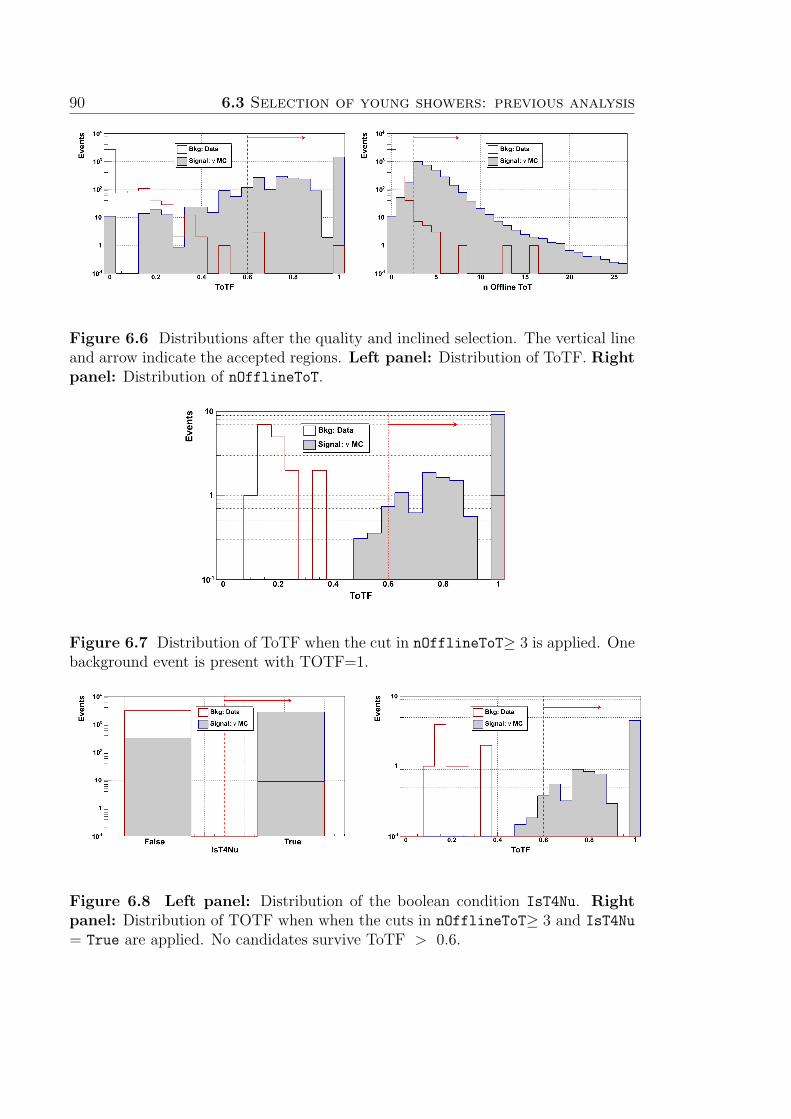
90 6.3 Selection of young showers: previous analysis
Figure 6.6 Distributions after the quality and inclined selection. The vertical lineand arrow indicate the accepted regions. Left panel: Distribution of ToTF. Rightpanel: Distribution of nOfflineToT.
Figure 6.7 Distribution of ToTF when the cut in nOfflineToT≥ 3 is applied. Onebackground event is present with TOTF=1.
Figure 6.8 Left panel: Distribution of the boolean condition IsT4Nu. Rightpanel: Distribution of TOTF when when the cuts in nOfflineToT≥ 3 and IsT4Nu
= True are applied. No candidates survive ToTF > 0.6.

6 Neutrino identification 91
Selection Efficiency
Quality
and 95.1%
Inclined
nOfflineToT 87.4%
IsT4Nu 85.0%
TOTF 84.1%
Table 6.1 Fraction of remaining yield after each selection cut.
The Old ES selection has advantages and disadvantages that are worth empha-
sizing here:
1. Advantages: The efficiency of selected neutrino Monte Carlo neutrino events
is high (∼ 84.1%).
2. Disadvantages: No background estimation is possible using the young selec-
tion variables. In particular, the requirement of 3 stations having ToT with
AoP>1.4 kills almost all events in the data sample so that no events are left to
extrapolate the behavior of the data sample distributions. Moreover, due to
the boolean nature of IsT4Nu, an extrapolation is complicated and unreliable.
We thus developed a new ES selection with efficiency similar to the Old ES, but
which allows an estimation of the background.
6.4 New Selection Strategy
As we have seen in Section 6.2 the variable area over peak AoP is a good dis-
criminant between showers induced by a τ decay and the hadronic background. In
Figure 6.9 we show how the AoP for 6-stations events changes as a function of the
station number ordered in time. It can be seen that for Earth-skimming neutrinos
the AoP is higher than for data in all stations. In the case of down-going neutrinos,
the AoP is also higher in general but there is a signicant difference between the
early and late part of the event. The reason for this was discussed and illustrated
in Figure 6.2.
In the bottom left panel of Figure 6.5 we have shown the distribution of the
AoP for the earliest station of every event. However we can exploit the fact that
events have multiple stations and average over them. It is worth noticing that we
have performed multiple tests using Fisher multivariate analysis combining different
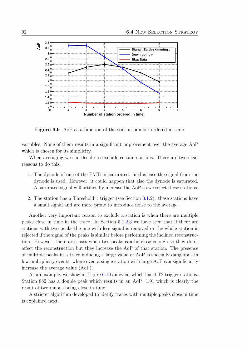
92 6.4 New Selection Strategy
Number of station ordered in time0 1 2 3 4 5 6 7
Ao
P
1
1.2
1.4
1.6
1.8
2
2.2
2.4
2.6
2.8
3
3.2
3.4
νSignal: Earth-skimming
νDown-going
Bkg: Data
Figure 6.9 AoP as a function of the station number ordered in time.
variables. None of them results in a significant improvement over the average AoP
which is chosen for its simplicity.
When averaging we can decide to exclude certain stations. There are two clear
reasons to do this.
1. The dynode of one of the PMTs is saturated: in this case the signal from the
dynode is used. However, it could happen that also the dynode is saturated.
A saturated signal will artificially increase the AoP so we reject these stations.
2. The station has a Threshold 1 trigger (see Section 3.1.2): these stations have
a small signal and are more prone to introduce noise to the average.
Another very important reason to exclude a station is when there are multiple
peaks close in time in the trace. In Section 5.1.2.3 we have seen that if there are
stations with two peaks the one with less signal is removed or the whole station is
rejected if the signal of the peaks is similar before performing the inclined reconstruc-
tion. However, there are cases when two peaks can be close enough so they don’t
affect the reconstruction but they increase the AoP of that station. The presence
of multiple peaks in a trace inducing a large value of AoP is specially dangerous in
low multiplicity events, where even a single station with large AoP can significantly
increase the average value 〈AoP〉.As an example, we show in Figure 6.10 an event which has 4 T2 trigger stations.
Station 882 has a double peak which results in an AoP=1.91 which is clearly the
result of two muons being close in time.
A stricter algorithm developed to idetify traces with multiple peaks close in time
is explained next.
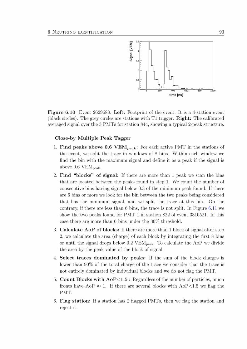
6 Neutrino identification 93
882
time [ns]0 200 400 600 800 1000
Sig
nal
[V
EM
]
0
0.5
1
1.5
2
2.5
Figure 6.10 Event 2629688. Left: Footprint of the event. It is a 4-station event(black circles). The grey circles are stations with T1 trigger. Right: The calibratedaveraged signal over the 3 PMTs for station 844, showing a typical 2-peak structure.
Close-by Multiple Peak Tagger
1. Find peaks above 0.6 VEMpeak: For each active PMT in the stations of
the event, we split the trace in windows of 8 bins. Within each window we
find the bin with the maximum signal and define it as a peak if the signal is
above 0.6 VEMpeak.
2. Find “blocks” of signal: If there are more than 1 peak we scan the bins
that are located between the peaks found in step 1. We count the number of
consecutive bins having signal below 0.3 of the minimum peak found. If there
are 6 bins or more we look for the bin between the two peaks being considered
that has the minimum signal, and we split the trace at this bin. On the
contrary, if there are less than 6 bins, the trace is not split. In Figure 6.11 we
show the two peaks found for PMT 1 in station 822 of event 3310521. In this
case there are more than 6 bins under the 30% threshold.
3. Calculate AoP of blocks: If there are more than 1 block of signal after step
2, we calculate the area (charge) of each block by integrating the first 8 bins
or until the signal drops below 0.2 VEMpeak. To calculate the AoP we divide
the area by the peak value of the block of signal.
4. Select traces dominated by peaks: If the sum of the block charges is
lower than 90% of the total charge of the trace we consider that the trace is
not entirely dominated by individual blocks and we do not flag the PMT.
5. Count Blocks with AoP<1.5 : Regardless of the number of particles, muon
fronts have AoP ≈ 1. If there are several blocks with AoP<1.5 we flag the
PMT.
6. Flag station: If a station has 2 flagged PMTs, then we flag the station and
reject it.
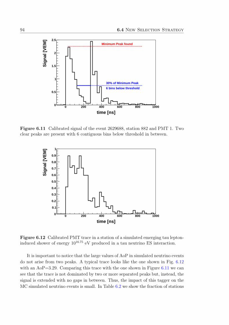
94 6.4 New Selection Strategy
time [ns]0 200 400 600 800 1000
Sig
nal
[V
EM
]
0
0.5
1
1.5
2
2.5Minimum Peak found
30% of Minimum Peak
6 bins below threshold
Figure 6.11 Calibrated signal of the event 2629688, station 882 and PMT 1. Twoclear peaks are present with 6 contiguous bins below threshold in between.
time [ns]0 200 400 600 800 1000
Sig
nal
[V
EM
]
0
0.1
0.2
0.3
0.4
0.5
0.6
0.7
0.8
0.9
1
Figure 6.12 Calibrated PMT trace in a station of a simulated emerging tau lepton-induced shower of energy 1016.75 eV produced in a tau neutrino ES interaction.
It is important to notice that the large values of AoP in simulated neutrino events
do not arise from two peaks. A typical trace looks like the one shown in Fig. 6.12
with an AoP=3.29. Comparing this trace with the one shown in Figure 6.11 we can
see that the trace is not dominated by two or more separated peaks but, instead, the
signal is extended with no gaps in between. Thus, the impact of this tagger on the
MC simulated neutrino events is small. In Table 6.2 we show the fraction of stations
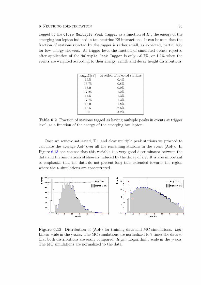
6 Neutrino identification 95
tagged by the Close Multiple Peak Tagger as a function of Eτ , the energy of the
emerging tau lepton induced in tau neutrino ES interactions. It can be seen that the
fraction of stations rejected by the tagger is rather small, as expected, particulary
for low energy showers. At trigger level the fraction of simulated events rejected
after application of the Multiple Peak Tagger is only ∼0.7%, or 1.2% when the
events are weighted according to their energy, zenith and decay height distributions.
log10 E[eV ] Fraction of rejected stations16.5 0.4%16.75 0.8%17.0 0.9%17.25 1.2%17.5 1.3%17.75 1.3%18.0 1.8%18.5 2.6%19 3.2%
Table 6.2 Fraction of stations tagged as having multiple peaks in events at triggerlevel, as a function of the energy of the emerging tau lepton.
Once we remove saturated, T1, and clear multiple peak stations we proceed to
calculate the average AoP over all the remaining stations in the event 〈AoP〉. In
Figure 6.13 one can see that this variable is a very good discriminator between the
data and the simulations of showers induced by the decay of a τ . It is also important
to emphasize that the data do not present long tails extended towards the region
where the ν simulations are concentrated.
Figure 6.13 Distribution of 〈AoP〉 for training data and MC simulations. Left:Linear scale in the y-axis. The MC simulations are normalized to 7 times the data sothat both distributions are easily compared. Right: Logarithmic scale in the y-axis.The MC simulations are normalized to the data.
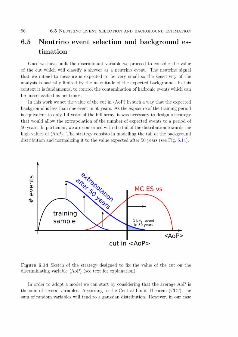
96 6.5 Neutrino event selection and background estimation
6.5 Neutrino event selection and background es-
timation
Once we have built the discriminant variable we proceed to consider the value
of the cut which will classify a shower as a neutrino event. The neutrino signal
that we intend to measure is expected to be very small so the sensitivity of the
analysis is basically limited by the magnitude of the expected background. In this
context it is fundamental to control the contamination of hadronic events which can
be missclassified as neutrinos.
In this work we set the value of the cut in 〈AoP〉 in such a way that the expected
background is less than one event in 50 years. As the exposure of the training period
is equivalent to only 1.4 years of the full array, it was necessary to design a strategy
that would allow the extrapolation of the number of expected events to a period of
50 years. In particular, we are concerned with the tail of the distribution towards the
high values of 〈AoP〉. The strategy consists in modelling the tail of the background
distribution and normalizing it to the value expected after 50 years (see Fig. 6.14).
MC ES νs
extrapolation
after 50 yearstraining sample
cut in <AoP>
# e
vent
s
1 bkg. eventin 50 years
<AoP>
Figure 6.14 Sketch of the strategy designed to fix the value of the cut on thediscriminating variable 〈AoP〉 (see text for explanation).
In order to adopt a model we can start by considering that the average AoP is
the sum of several variables. According to the Central Limit Theorem (CLT), the
sum of random variables will tend to a gaussian distribution. However, in our case

6 Neutrino identification 97
Figure 6.15 Distribution of the average Area over Peak in the Training data forevents with 4 stations or more. The mean 〈AoP〉 of the distribution is indicated witha vertical line. A gaussian fit between [〈AoP〉 − RMS, 〈AoP〉 + RMS] is performedand shown in thick black. In grey we show the extrapolation of the fit. Towards theright the distribution falls slower than predicted by the gaussian fit.
the sum is done over a small number of stations and this number is not enough
to obtain a gaussian distribution. As can be seen in Figure 6.15 the tail of the
distribution falls slower than predicted by a gaussian fit. It is interesting to note
that the gaussian prediction works well (poorly) for fluctuations towards low (high)
values of 〈AoP〉. This is somewhat expected, as the tail towards high 〈AoP〉 can be
driven by fluctuations in only one station, where the CLT does not apply, while the
tail towards low 〈AoP〉 arises from the combined effect of all stations.
For the reasons above we adopted an exponential model which falls slower than
the gaussian, and describes well the data.
N(〈AoP〉) = eA−B〈AoP〉 (6.1)
where N(〈AoP〉) is the number of events in a bin of width ∆〈AoP〉. Using logarith-
mic scale for the y-axis this model is a line where B is the slope.
Using this functional form we fit over the tail of the distribution in the [1σ, 3σ]
region 1. The result is shown in Figure 6.16.
We test the fit quality in two ways. First, we calculate the statistics χ2 divided
1This notation denominates the region in the interval [〈AoP〉+ 1RMS, 〈AoP〉+ 3RMS].
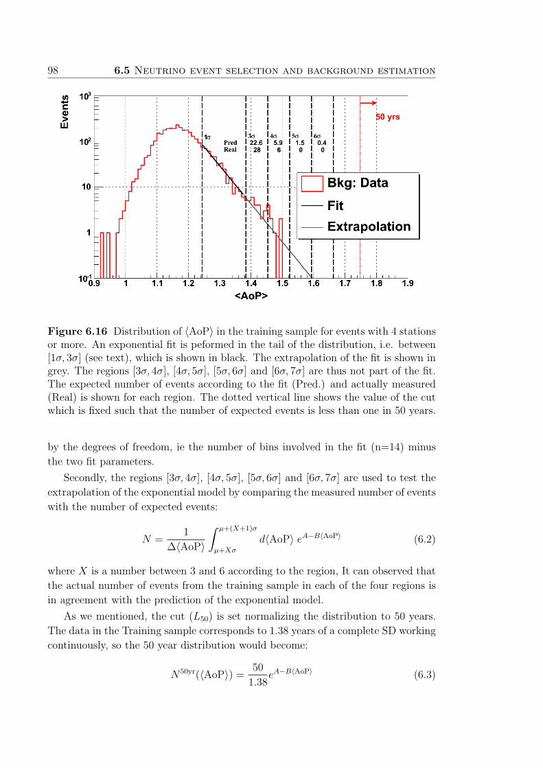
98 6.5 Neutrino event selection and background estimation
Figure 6.16 Distribution of 〈AoP〉 in the training sample for events with 4 stationsor more. An exponential fit is peformed in the tail of the distribution, i.e. between[1σ, 3σ] (see text), which is shown in black. The extrapolation of the fit is shown ingrey. The regions [3σ, 4σ], [4σ, 5σ], [5σ, 6σ] and [6σ, 7σ] are thus not part of the fit.The expected number of events according to the fit (Pred.) and actually measured(Real) is shown for each region. The dotted vertical line shows the value of the cutwhich is fixed such that the number of expected events is less than one in 50 years.
by the degrees of freedom, ie the number of bins involved in the fit (n=14) minus
the two fit parameters.
Secondly, the regions [3σ, 4σ], [4σ, 5σ], [5σ, 6σ] and [6σ, 7σ] are used to test the
extrapolation of the exponential model by comparing the measured number of events
with the number of expected events:
N =1
∆〈AoP〉
∫ µ+(X+1)σ
µ+Xσ
d〈AoP〉 eA−B〈AoP〉 (6.2)
where X is a number between 3 and 6 according to the region, It can observed that
the actual number of events from the training sample in each of the four regions is
in agreement with the prediction of the exponential model.
As we mentioned, the cut (L50) is set normalizing the distribution to 50 years.
The data in the Training sample corresponds to 1.38 years of a complete SD working
continuously, so the 50 year distribution would become:
N50yr(〈AoP〉) = 50
1.38eA−B〈AoP〉 (6.3)
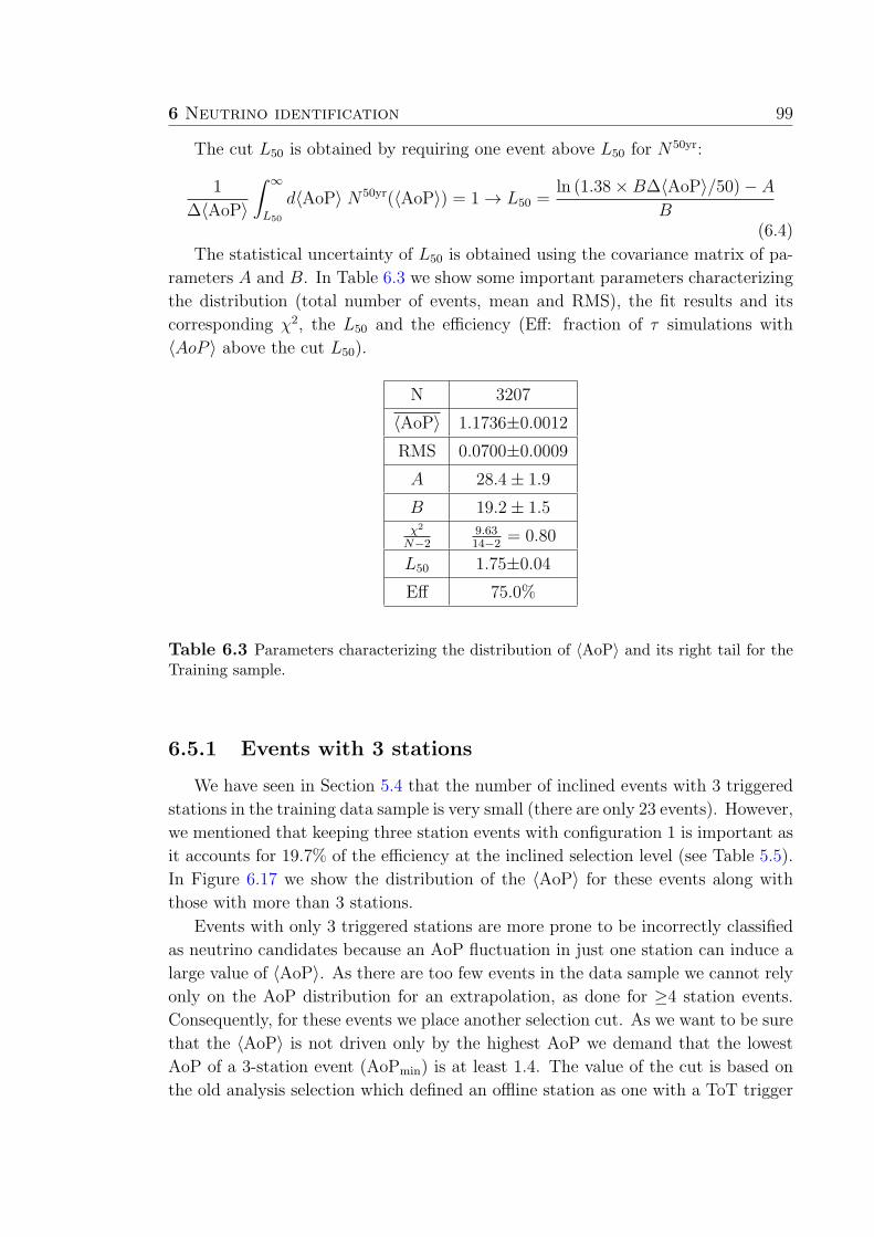
6 Neutrino identification 99
The cut L50 is obtained by requiring one event above L50 for N50yr:
1
∆〈AoP〉
∫ ∞
L50
d〈AoP〉 N50yr(〈AoP〉) = 1 → L50 =ln (1.38× B∆〈AoP〉/50)− A
B(6.4)
The statistical uncertainty of L50 is obtained using the covariance matrix of pa-
rameters A and B. In Table 6.3 we show some important parameters characterizing
the distribution (total number of events, mean and RMS), the fit results and its
corresponding χ2, the L50 and the efficiency (Eff: fraction of τ simulations with
〈AoP 〉 above the cut L50).
N 3207
〈AoP〉 1.1736±0.0012
RMS 0.0700±0.0009
A 28.4± 1.9
B 19.2± 1.5χ2
N−29.6314−2
= 0.80
L50 1.75±0.04
Eff 75.0%
Table 6.3 Parameters characterizing the distribution of 〈AoP〉 and its right tail for theTraining sample.
6.5.1 Events with 3 stations
We have seen in Section 5.4 that the number of inclined events with 3 triggered
stations in the training data sample is very small (there are only 23 events). However,
we mentioned that keeping three station events with configuration 1 is important as
it accounts for 19.7% of the efficiency at the inclined selection level (see Table 5.5).
In Figure 6.17 we show the distribution of the 〈AoP〉 for these events along with
those with more than 3 stations.
Events with only 3 triggered stations are more prone to be incorrectly classified
as neutrino candidates because an AoP fluctuation in just one station can induce a
large value of 〈AoP〉. As there are too few events in the data sample we cannot rely
only on the AoP distribution for an extrapolation, as done for ≥4 station events.
Consequently, for these events we place another selection cut. As we want to be sure
that the 〈AoP〉 is not driven only by the highest AoP we demand that the lowest
AoP of a 3-station event (AoPmin) is at least 1.4. The value of the cut is based on
the old analysis selection which defined an offline station as one with a ToT trigger
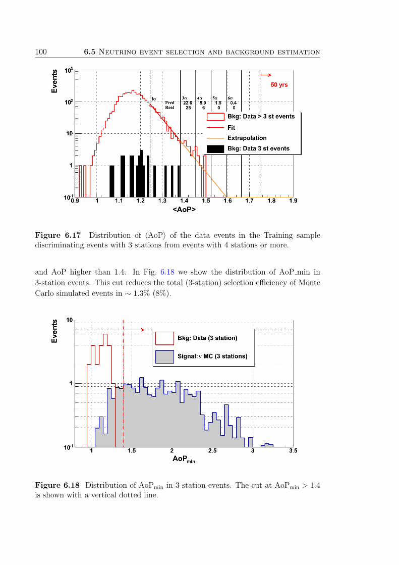
100 6.5 Neutrino event selection and background estimation
Figure 6.17 Distribution of 〈AoP〉 of the data events in the Training samplediscriminating events with 3 stations from events with 4 stations or more.
and AoP higher than 1.4. In Fig. 6.18 we show the distribution of AoP min in
3-station events. This cut reduces the total (3-station) selection efficiency of Monte
Carlo simulated events in ∼ 1.3% (8%).
Figure 6.18 Distribution of AoPmin in 3-station events. The cut at AoPmin > 1.4is shown with a vertical dotted line.
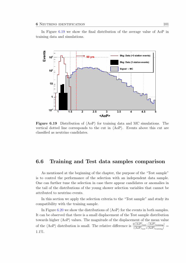
6 Neutrino identification 101
In Figure 6.19 we show the final distribution of the average value of AoP in
training data and simulations.
Figure 6.19 Distribution of 〈AoP〉 for training data and MC simulations. Thevertical dotted line corresponds to the cut in 〈AoP〉. Events above this cut areclassified as neutrino candidates.
6.6 Training and Test data samples comparison
As mentioned at the beginning of the chapter, the purpose of the “Test sample”
is to control the performance of the selection with an independent data sample.
One can further tune the selection in case there appear candidates or anomalies in
the tail of the distributions of the young shower selection variables that cannot be
attributed to neutrino events.
In this section we apply the selection criteria to the “Test sample” and study its
compatibility with the training sample.
In Figure 6.20 we show the distributions of 〈AoP〉 for the events in both samples.
It can be observed that there is a small displacement of the Test sample distribution
towards higher 〈AoP〉 values. The magnitude of the displacement of the mean value
of the 〈AoP〉 distribution is small. The relative difference is2(〈AoP〉test−〈AoP〉training)
(〈AoP〉test+〈AoP〉training)=
1.1%.
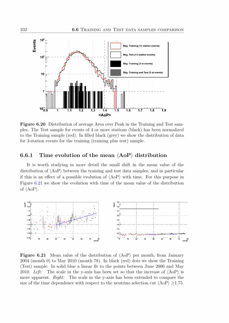
102 6.6 Training and Test data samples comparison
Figure 6.20 Distribution of average Area over Peak in the Training and Test sam-ples. The Test sample for events of 4 or more stations (black) has been normalizedto the Training sample (red). In filled black (grey) we show the distribution of datafor 3-station events for the training (training plus test) sample.
6.6.1 Time evolution of the mean 〈AoP〉 distribution
It is worth studying in more detail the small shift in the mean value of the
distribution of 〈AoP〉 between the training and test data samples, and in particular
if this is an effect of a possible evolution of 〈AoP〉 with time. For this purpose in
Figure 6.21 we show the evolution with time of the mean value of the distribution
of 〈AoP〉.
Figure 6.21 Mean value of the distribution of 〈AoP〉 per month, from January2004 (month 0) to May 2010 (month 78). In black (red) dots we show the Training(Test) sample. In solid blue a linear fit to the points between June 2006 and May2010. Left: The scale in the y-axis has been set so that the increase of 〈AoP〉 ismore apparent. Right: The scale in the y-axis has been extended to compare thesize of the time dependence with respect to the neutrino selection cut 〈AoP〉 ≥1.75.

6 Neutrino identification 103
Performing a fit between June 2006 and May 2010 we find that the 〈AoP〉increases with a slope of ∼ (0.65 ± 0.15)%
yr. We should however emphasize that
the increase is small when compared to the position of the neutrino selection cut,
〈AoP〉 ≥1.75 (see Fig. 6.21).
We have tested whether this increase also happens for showers with smaller zenith
angles. This was achieved by placing a different cut on the velocity of the signal at
ground, namely 0.31nms
< 〈V 〉 < 0.32nms
(similar to 70 < θ < 75) instead of the
nominal 0.29nms
< 〈V 〉 < 0.31nms. The slope of 〈AoP〉 is compatible with 0 in this
case.
6.6.2 Compatibility of the tails of the distributions in the
Training and Test samples
An important test is the compatibility between the tails of the distributions of
〈AoP〉 in both samples. In Figure 6.22 we show the distribution of the Test sample
along with the corresponding fit to the tail (see Figure 6.17 to compare with the
training sample). In Table 6.4 we show the slope of the fit along with the other
parameters characterizing the distribution (see Table 6.3 to compare with Training
sample).
Figure 6.22 Distribution of average Area over Peak for the Test sample.
The distribution of 〈AoP〉 in the Test sample differs from the Training sample
both in the mean value and in the slope of the linear fit to the tail. The shift in

104 6.6 Training and Test data samples comparison
N 4660
〈AoP〉 1.1866±0.0011
RMS 0.0725±0.0008
A 26.8± 1.6
B 17.5± 1.2χ2
N−29.4314−2
= 0.79
L50 1.82±0.04
Eff 71.3%
Table 6.4 Parameters of the distribution of 〈AoP〉 for the Test sample.
mean value of 〈AoP〉 is small (+1.1%), but significant (8σ) 2. The change in slope
is larger (9.3%), but compatible within uncertainties (0.9 std).
The value of the cut L50 is based on the extrapolation of the linear fit to the
tail of the distribution of 〈AoP〉. The uncertainty on the A and B propagates to an
uncertainty of 0.04 (2%) on L50.
The change in L50 due to the shift in mean value is small, it amounts to ∼0.013 (0.7%). The total change in L50 is 0.07 (4%). This means that the dominant
effect is not the shift in mean value, but the large uncertainty in the fit.
We have performed an extra check to confirm that the uncertainties on the
slopes are reasonable. We have constructed two “clone” samples dividing the total
sample (Training + Test) in events with even and odd event numbers. With this
construction the two samples are equally influenced by the time evolution of 〈AoP〉shown in Fig. 6.21. Performing a fit to the tails of the cloned distributions, the slopes
are 17.8 ± 1.2 and 19.1 ± 1.2 respectively, showing again a rather large difference
(7%) but again compatible within uncertainties.
6.6.3 Remarks and Conclusions
1. The distribution of the young shower identification variable 〈AoP〉 in the Test
sample shows a small displacement of +1.1% with respect to the Training
sample.
2. The tails of the Training and Test distributions are compatible within the
statistical uncertainties of their corresponding exponential fits. The difference
in slopes translates into a difference on the cut on 〈AoP〉 of +0.07 (+4%).
2The disagreement masured in standard deviations (σ) between two variables v1 ± σv1 andv2 ± σv2
is calculated as v1−v2√σ2v1
+σ2v2
, In the case of the 〈AoP〉 the uncertainty is σ(〈AoP〉) ≡RMS(〈AoP〉)√
Ni
.

6 Neutrino identification 105
3. Since the purpose of the Test sample was to allow us to refine the cuts if
needed, we use as the final cut on 〈AoP〉 the one that results from the Test
sample, namely 〈AoP〉 ≥1.82 instead of 〈AoP〉 ≥1.75. The reasons to do this
is that this sample is closer in time to the search sample and the cut is higher
(more conservative) that the one derived with the Training sample.
6.7 Summary
In Table 6.5 we display the criteria used to classify an event as a neutrino once
it has passed the quality and inclined selections.
nStation ≥ 4 nStation = 3
Young 〈AoP〉 ≥1.82
Showers - AoP min>1.4
Table 6.5 Observables and numerical values of cuts applied to select young showers.
In Table 6.6 we display the efficiency after applying the selection criteria.
nStation ≥ 4 nStation = 3 Total
Quality
and 65.5% 19.7% 85.2%
Inclined
〈AoP〉 ≥1.82 55.4% 15.9% 71.3%
AoP min>1.4 - 14.6% 70.0%
Table 6.6 Selection efficiency. In the first column we give the selection criteria applied.We divide the samples according to the number of stations.
In Table 6.7 we compare the Training and Test samples when applying the quality
and inclined selection. None of the events pass the young selection criteria.
nStation ≥ 4 nStation = 3 Total
Training 3207 23 3230
Test 4660 21 4681
Table 6.7 Number of data events after the quality and inclined selection.


7Detector efficiency andexposure
In this chapter we study in detail the neutrino identification efficiency using
the algorithms presented in the previous two sections. In Section 7.1 we present
the detector efficiency and introduce the concept of effective area. In Section 7.2 we
discuss the procedure to calculate, given a diffuse flux, the expected number of events
at the surface detector. This derivation allow us to define the exposure which is the
physical magnitude that summarizes the potential for discovery of the experiment.
Finally, we examine and quantify the systematic uncertainties associated with the
exposure determination.
7.1 Detector efficiency
In order to develop some intuition about the behaviour and performance of the
neutrino identification method, it is useful first to consider the idealized case of
an infinite array. In practice, an “infinite array” means an array large enough so
that all simulated showers are completely contained. In Sec. 7.1.2, the case of the
real detector with finite size is discussed, where it is important to consider the
contribution of events that fall in the border and are only partially contained.
7.1.1 Infinite detector efficiency
The MC generated showers initiated by τ decays (Section 4.2.2) were simulated
in the central region of a detector composed of 50×50 stations disposed in a per-
fectly hexagonal array with 1500 m of separation, very similar to the real SD array
(although this one is not perfectly regular and its size is smaller).
107
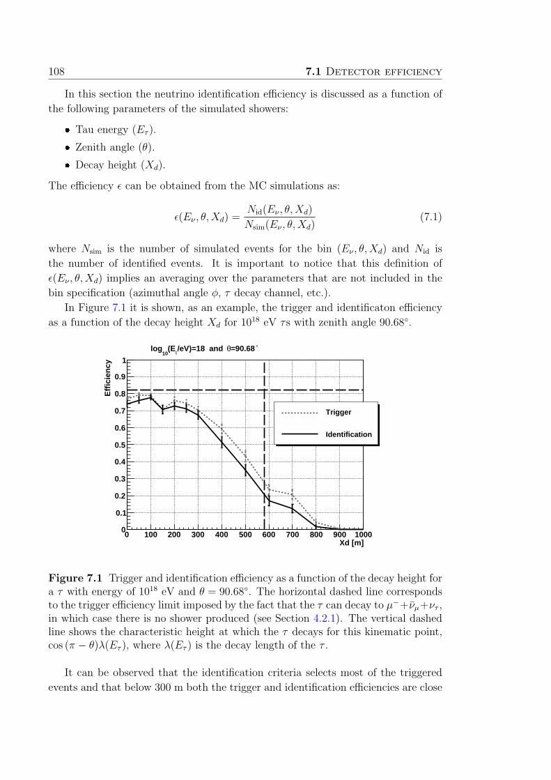
108 7.1 Detector efficiency
In this section the neutrino identification efficiency is discussed as a function of
the following parameters of the simulated showers:
❼ Tau energy (Eτ ).
❼ Zenith angle (θ).
❼ Decay height (Xd).
The efficiency ǫ can be obtained from the MC simulations as:
ǫ(Eν , θ,Xd) =Nid(Eν , θ,Xd)
Nsim(Eν , θ,Xd)(7.1)
where Nsim is the number of simulated events for the bin (Eν , θ,Xd) and Nid is
the number of identified events. It is important to notice that this definition of
ǫ(Eν , θ,Xd) implies an averaging over the parameters that are not included in the
bin specification (azimuthal angle φ, τ decay channel, etc.).
In Figure 7.1 it is shown, as an example, the trigger and identificaton efficiency
as a function of the decay height Xd for 1018 eV τs with zenith angle 90.68.
Xd [m]0 100 200 300 400 500 600 700 800 900 1000
Eff
icie
ncy
0
0.1
0.2
0.3
0.4
0.5
0.6
0.7
0.8
0.9
1
Trigger
Identification
=90.68θ/eV)=18 and τ(E10
log °
Figure 7.1 Trigger and identification efficiency as a function of the decay height fora τ with energy of 1018 eV and θ = 90.68. The horizontal dashed line correspondsto the trigger efficiency limit imposed by the fact that the τ can decay to µ−+νµ+ντ ,in which case there is no shower produced (see Section 4.2.1). The vertical dashedline shows the characteristic height at which the τ decays for this kinematic point,cos (π − θ)λ(Eτ ), where λ(Eτ ) is the decay length of the τ .
It can be observed that the identification criteria selects most of the triggered
events and that below 300 m both the trigger and identification efficiencies are close
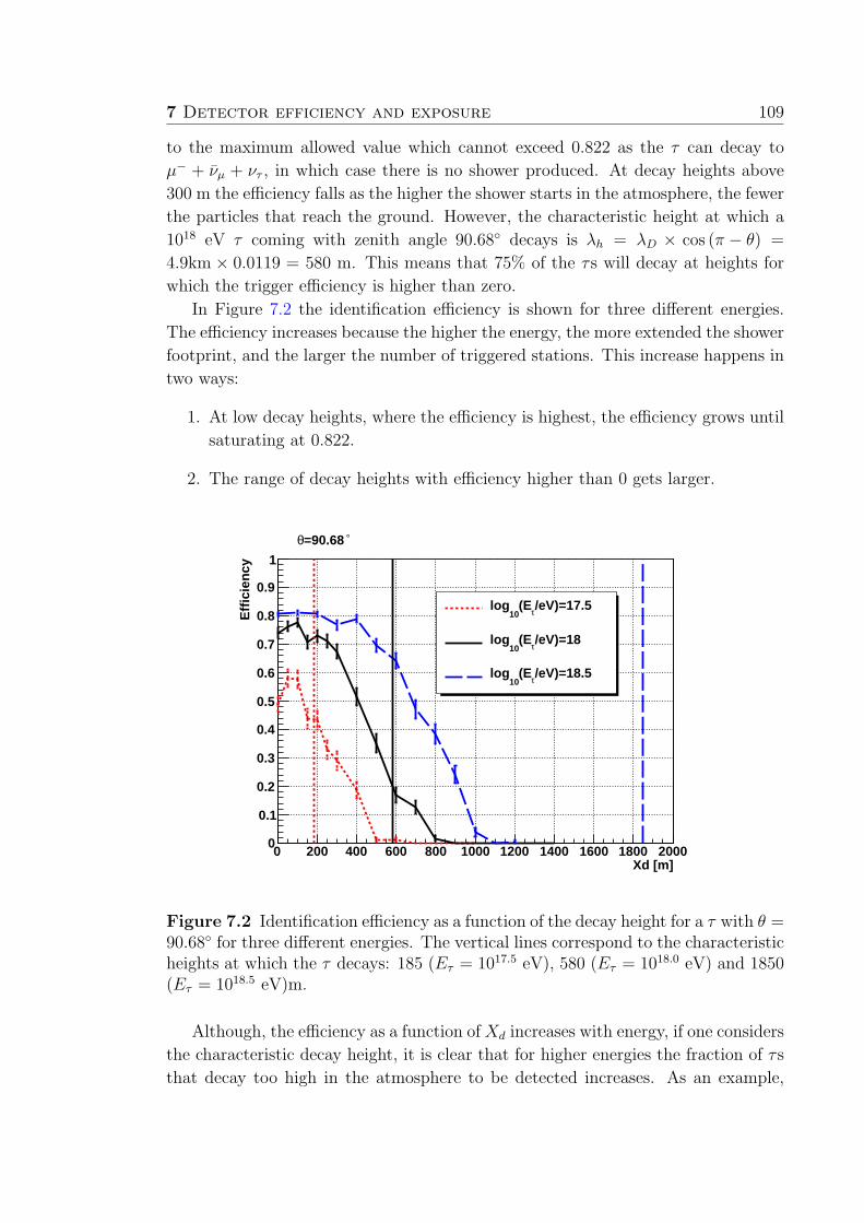
7 Detector efficiency and exposure 109
to the maximum allowed value which cannot exceed 0.822 as the τ can decay to
µ− + νµ + ντ , in which case there is no shower produced. At decay heights above
300 m the efficiency falls as the higher the shower starts in the atmosphere, the fewer
the particles that reach the ground. However, the characteristic height at which a
1018 eV τ coming with zenith angle 90.68 decays is λh = λD × cos (π − θ) =
4.9km × 0.0119 = 580 m. This means that 75% of the τs will decay at heights for
which the trigger efficiency is higher than zero.
In Figure 7.2 the identification efficiency is shown for three different energies.
The efficiency increases because the higher the energy, the more extended the shower
footprint, and the larger the number of triggered stations. This increase happens in
two ways:
1. At low decay heights, where the efficiency is highest, the efficiency grows until
saturating at 0.822.
2. The range of decay heights with efficiency higher than 0 gets larger.
Xd [m]0 200 400 600 800 1000 1200 1400 1600 1800 2000
Eff
icie
ncy
0
0.1
0.2
0.3
0.4
0.5
0.6
0.7
0.8
0.9
1
/eV)=17.5τ(E10
log
/eV)=18τ(E10
log
/eV)=18.5τ(E10
log
=90.68θ °
Figure 7.2 Identification efficiency as a function of the decay height for a τ with θ =90.68 for three different energies. The vertical lines correspond to the characteristicheights at which the τ decays: 185 (Eτ = 1017.5 eV), 580 (Eτ = 1018.0 eV) and 1850(Eτ = 1018.5 eV)m.
Although, the efficiency as a function ofXd increases with energy, if one considers
the characteristic decay height, it is clear that for higher energies the fraction of τs
that decay too high in the atmosphere to be detected increases. As an example,
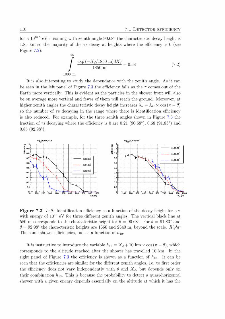
110 7.1 Detector efficiency
for a 1018.5 eV τ coming with zenith angle 90.68 the characteristic decay height is
1.85 km so the majority of the τs decay at heights where the efficiency is 0 (see
Figure 7.2):∞∫
1000 m
exp (−Xd/1850 m)dXd
1850 m= 0.58 (7.2)
It is also interesting to study the dependance with the zenith angle. As it can
be seen in the left panel of Figure 7.3 the efficiency falls as the τ comes out of the
Earth more vertically. This is evident as the particles in the shower front will also
be on average more vertical and fewer of them will reach the ground. Moreover, at
higher zenith angles the characteristic decay height increases λh = λD × cos (π − θ)
so the number of τs decaying in the range where there is identification efficiency
is also reduced. For example, for the three zenith angles shown in Figure 7.3 the
fraction of τs decaying where the efficiency is 0 are 0.21 (90.68), 0.68 (91.83) and
0.85 (92.98).
Xd [m]0 100 200 300 400 500 600 700 800 900 1000
Eff
icie
ncy
0
0.1
0.2
0.3
0.4
0.5
0.6
0.7
0.8
0.9
1
°=90.68θ
°=91.83θ
°=92.98θ
/eV)=18τ(E10
log
[m]10h0 100 200 300 400 500 600 700 800 900 1000
Eff
icie
ncy
0
0.1
0.2
0.3
0.4
0.5
0.6
0.7
0.8
0.9
1°
=90.68θ
°=91.83θ
°=92.98θ
/eV)=18τ(E10
log
Figure 7.3 Left: Identification efficiency as a function of the decay height for a τwith energy of 1018 eV for three different zenith angles. The vertical black line at580 m corresponds to the characteristic height for θ = 90.68. For θ = 91.83 andθ = 92.98 the characteristic heights are 1560 and 2540 m, beyond the scale. Right:The same shower efficiencies, but as a function of h10.
It is instructive to introduce the variable h10 ≡ Xd + 10 km× cos (π − θ), which
corresponds to the altitude reached after the shower has travelled 10 km. In the
right panel of Figure 7.3 the efficiency is shown as a function of h10. It can be
seen that the efficiencies are similar for the different zenith angles, i.e. to first order
the efficiency does not vary independently with θ and Xd, but depends only on
their combination h10. This is because the probability to detect a quasi-horizontal
shower with a given energy depends essentially on the altitude at which it has the
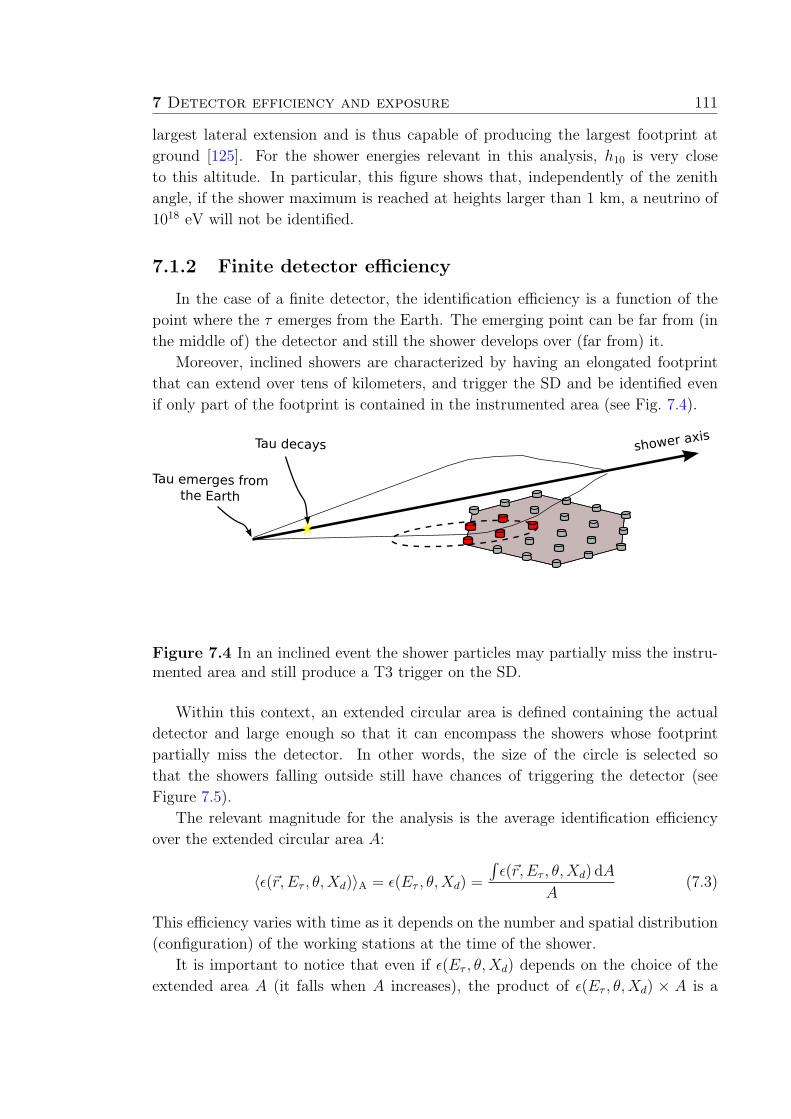
7 Detector efficiency and exposure 111
largest lateral extension and is thus capable of producing the largest footprint at
ground [125]. For the shower energies relevant in this analysis, h10 is very close
to this altitude. In particular, this figure shows that, independently of the zenith
angle, if the shower maximum is reached at heights larger than 1 km, a neutrino of
1018 eV will not be identified.
7.1.2 Finite detector efficiency
In the case of a finite detector, the identification efficiency is a function of the
point where the τ emerges from the Earth. The emerging point can be far from (in
the middle of) the detector and still the shower develops over (far from) it.
Moreover, inclined showers are characterized by having an elongated footprint
that can extend over tens of kilometers, and trigger the SD and be identified even
if only part of the footprint is contained in the instrumented area (see Fig. 7.4).
shower axis
Tau emerges fromthe Earth
Tau decays
Figure 7.4 In an inclined event the shower particles may partially miss the instru-mented area and still produce a T3 trigger on the SD.
Within this context, an extended circular area is defined containing the actual
detector and large enough so that it can encompass the showers whose footprint
partially miss the detector. In other words, the size of the circle is selected so
that the showers falling outside still have chances of triggering the detector (see
Figure 7.5).
The relevant magnitude for the analysis is the average identification efficiency
over the extended circular area A:
〈ǫ(~r, Eτ , θ,Xd)〉A = ǫ(Eτ , θ,Xd) =
∫ǫ(~r, Eτ , θ,Xd) dA
A(7.3)
This efficiency varies with time as it depends on the number and spatial distribution
(configuration) of the working stations at the time of the shower.
It is important to notice that even if ǫ(Eτ , θ,Xd) depends on the choice of the
extended area A (it falls when A increases), the product of ǫ(Eτ , θ,Xd) × A is a

112 7.1 Detector efficiency
Position [Km]-40 -30 -20 -10 0 10 20 30 40
Position [Km]
-40
-30
-20
-10
0
10
20
30
40
1
3
2
4
Figure 7.5 Example of a simulated shower, initiated by the decay of a τ , in four dif-ferent positions over a finite detector (shadowed area) corresponding to 1 November2007. The arrows indicate the direction of the shower, the points represent the idealand infinite array of stations and the circunference the extended area (see text).Solid (open) symbols correspond to stations of the simulated shower which have aT2 local trigger and which are (not) active in the reference configuration. Roundsymbols indicate showers which are identified as neutrinos and square symbols thosewhich are not. In case 1 the shower is fully contained and identified as a neutrino.In case 2 the shower is completely out and, consequently, does not trigger the realdetector. In case 3 (4) the shower is partially contained and triggers the SD, howeverit is (not) identified as a neutrino because, by chance, the stations with higher areaover peak fall inside (outside) the real detector.
constant which defines an intrinsic property called effective area Aeff :
Aeff(Eτ , θ,Xd) =
∫
A
ǫ(~r, Eτ , θ,Xd) dA (7.4)
This area represents the equivalent surface of a 100% efficient detector. In princi-

7 Detector efficiency and exposure 113
ple, to calculate this magnitude, one should perform the complete set of simulations
from the decay to the response of the detector for every configuration. However,
this is impractical and it would require a number of simulations impossible to be
carried out. For this reason, it was decided to follow a different approach in which
the simulations produced in the infinite array are reused to calculate the identifi-
cation efficiencies in all possible configurations of the real SD. The barycenter of
each shower simulated over the ideal array is randomly located over the extended
circular area. The stations of the simulated events that do not match an active
station of the finite array are discarded (see Fig. 7.5). In this way one has the event
that would be obtained if the simulation would have been performed over the actual
detector. Using only the selected stations, the trigger conditions are reevaluated
and, if satisfied, the global variables are recomputed and the inclined and young
selection cuts are applied. In Fig. 7.5 it is summarized, as an example, the results of
possible reevaluations of a single event which is identified as a neutrino in the case
of an infinite array.
The ratio of identified events over the total events defines the identification effi-
ciency ǫ(Eν , θ,Xd, t) of the configuration:
ǫ(Eτ , θ,Xd, t) =Nid(Eτ , θ,Xd, t)
Nsim(Eτ , θ,Xd)(7.5)
where the dependence on t reminds that the efficiency varies from configuration to
configuration.
Aeff(Eτ , θ,Xd, t) is obtained by multiplying by the surface of the extended area A:
Aeff(Eν , θ,Xd, t) = ǫ(Eτ , θ,Xd, t)× A (7.6)
7.2 Exposure
7.2.1 Exposure definition
We define the diffuse exposure E as the magnitude that when convoluted with
the diffuse ν flux results in the number of expected events.
Nexp =
∫ Emax
Emin
Φ(Eν) E(Eν) dEν (7.7)
It is, in a way, the magnitude that shows how good an experiment is, as it
determines which are the fluxes one could be able to measure and which are not.
Inverting the problem, if one observes a number of events n, one has to divide by
the exposure in order to derive the incident flux at Earth.
In Section 4.3 it has been discussed that the number of expected events per unit

114 7.2 Exposure
of time and area is:
dNexp
dtdA=
∫
dEν
∫
dEτ
∫
dΩ
∫
dXd Φ(Eν) f(Eτ |θ, Eν)h(Xd|Eτ , θ) | cos (θ)| ε(Eτ , θ,Xd)
(7.8)
where f(Eτ |θ, Eν) and h(Xd|Eτ , θ) are the probability density functions defined in
Section 4.3.
The number of expected events per unit of time is obtained by considering the
effective area Aeff(Eτ , θ,Xd, t), defined in equation 7.6:
dNexp
dt=
∫
dEν
∫
dEτ
∫
dΩ
∫
dXd Φ(Eν) f(Eτ |θ, Eν)h(Xd|Eτ , θ) | cos (θ)| Aeff(Eτ , θ,Xd, t)
(7.9)
where we have included the time dependence of Aeff (equation 7.6).
Consequently, considering equations 7.7 and 7.9 we have that the exposure is:
E(Eν) =
∫
dt
∫
dEτ
∫
dΩ
∫
dXd f(Eτ |θ, Eν)h(Xd|Eτ , θ) | cos θ| Aeff(Eτ , θ,Xd, t)
(7.10)
Integrating in φ we obtain:
E(Eν) =2π
∫
dt
∫
dEτ
∫
d cos θ
∫
dXd f(Eτ |θ, Eν)h(Xd|Eτ , θ) | cos θ| Aeff(Eτ , θ,Xd, t)
(7.11)
7.2.2 Temporal evolution of the SD
Calculating the time integrated exposure of a real detector is not simple. The SD
was in construction until the end of 2008. Moreover, the number of active stations
changed not only while it was being constructed but also because of temporal failures
or maintenance periods. Therefore, it was necessary to develop a method capable
of contemplating the temporal evolution.
The state of the detector is monitored every second via the trigger T2 frequency of
all stations that indicates which are working correctly. This information is translated
into files which register all configurations (set of active stations) of the SD with a
time resolution of 1 second. Ideally, the exposure would have to be evaluated over
all configurations and integrated over the lapse of time corresponding to each one.
As it is not possible to consider individually this huge number of configurations,
the period from January 2004 to December 2012 (3287 days) is divided into 1095
sub-periods of 3 days and for each sub-period a reference configuration is selected.
The live time assigned to each of these configurations corresponds to the duration
the array has a number of stations higher or equal than the reference one.
For each period, it is not obvious which of the many configurations is to be
chosen as the representative one. In order to deal with this problem we make
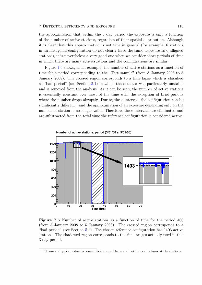
7 Detector efficiency and exposure 115
the approximation that within the 3 day period the exposure is only a function
of the number of active stations, regardless of their spatial distribution. Although
it is clear that this approximation is not true in general (for example, 6 stations
in an hexagonal configuration do not clearly have the same exposure as 6 alligned
stations), it is nevertheless a very good one when we consider short periods of time
in which there are many active stations and the configurations are similar.
Figure 7.6 shows, as an example, the number of active stations as a function of
time for a period corresponding to the “Test sample” (from 3 January 2008 to 5
January 2008). The crossed region corresponds to a time lapse which is classified
as “bad period” (see Section 5.1) in which the detector was particularly unstable
and is removed from the analysis. As it can be seen, the number of active stations
is essentially constant over most of the time with the exception of brief periods
where the number drops abruptly. During these intervals the configuration can be
significantly different 1 and the approximation of an exposure depending only on the
number of station is no longer valid. Therefore, these intervals are eliminated and
are substracted from the total time the reference configuration is considered active.
Figure 7.6 Number of active stations as a function of time for the period 488(from 3 January 2008 to 5 January 2008). The crossed region corresponds to a“bad period” (see Section 5.1). The chosen reference configuration has 1403 activestations. The shadowed region corresponds to the time ranges actually used in this3-day period.
1These are typically due to communication problems and not to local failures at the stations.

116 7.2 Exposure
The representative configuration is chosen so that the productN×T is maximum,
where N is a given number of active stations and T is the time in which the detector
has a number of stations equal or higher than N . In this way, each 3-day period
is analysed, and a configuration selected maximizing the mentioned criterion. If
there is more than one configuration satisfying the criterion, one keeps the earliest.
There is no difference between using this configuration or the next one under the
approximation we are working with.
This method allows to obtain a lower limit to the exposure of the detector as
the number of active stations is underestimated. The systematic uncertainty of this
approach is studied by analysing the differences produced when selecting a reference
configuration for different number of days. The result is that the effect is of the order
of 1%, much lower that other uncertainties discussed in Sec. 7.2.5.
7.2.3 Exposure calculation
In this section we explain how the calculation of the exposure is done. In the
previous section we have explained how to obtain a reference configuration for a
3-day period and in Section 7.1.2 we have explained how to obtain the effective
area, Aeff. We will use the effective areas corresponding to configuration 488 (from
3 January 2008 to 5 January 2008) to illustrate the procedure.
In order to perform an integration over the parameter space of Eτ , θ and Xd, thefirst step is to complete the cubic grid defined in Section 4.3. We have mentionedthat there are regions in the parameter space that contribute more to the eventrate than others so we have sampled them with a smaller step. For energies below1018 eV and θ < 94 we have simulated showers with a separation of ∆Xd = 50 mwhile higher energies or higher zenith angles the parameter space is sampled with∆Xd = 100 m. When the step is ∆Xd = 100 m, the ∆Xd = 50 m point is obtainedby a linear interpolation. For example:
Aeff(50 m) =Aeff(0 m) +Aeff(100 m)
2for log10 (Eτ/eV) = 18.5 and θ = 90.68 (7.12)
Also, for energies below 1018 eV we have sampled the parameter space with∆ log10(Eτ/eV) = 0.25 while for higher energies the separation is ∆ log10(Eτ/eV) =0.5. When not available, the ∆ log10(Eτ/eV) = 0.25 point is obtained by a linearinterpolation in log scale. For example:
Aeff(1018.25 eV) =
Aeff(1018 eV) +Aeff(10
18.5eV)
2for θ = 90.68 and Xd = 50 m (7.13)
Once that we have a cubic grid the effective area at any point (Eτ , θ, Xd)is obtained by a trilinear interpolation where the 8 vertices around the point are
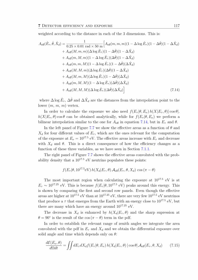
7 Detector efficiency and exposure 117
weighted according to the distance in each of the 3 dimensions. This is:
Aeff(Eτ , θ, Xd) =1
0.25× 0.01 rad× 50 m
[
Aeff(m,m,m)(1−∆ log Eτ )(1−∆θ)(1−∆Xd)
+Aeff(M,m,m)(∆ log Eτ )(1−∆θ)(1−∆Xd)
+Aeff(m,M,m)(1−∆ log Eτ )(∆θ)(1−∆Xd)
+Aeff(m,m,M)(1−∆ log Eτ )(1−∆θ)(∆Xd)
+Aeff(M,M,m)(∆ log Eτ )(∆θ)(1−∆Xd)
+Aeff(M,m,M)(∆ log Eτ )(1−∆θ)(∆Xd)
+Aeff(m,M,M)(1−∆ log Eτ )(∆θ)(∆Xd)
+Aeff(M,M,M)(∆ log Eτ )(∆θ)(∆Xd)]
(7.14)
where ∆ log Eτ , ∆θ and ∆Xd are the distances from the interpolation point to the
lower (m, m, m) vertex.
In order to calculate the exposure we also need f(Eτ |θ, Eν)h(X|Eτ , θ)| cos θ|.h(X|Eτ , θ) cos θ can be obtained analytically, while for f(Eτ |θ, Eν) we perform a
bilinear interpolation similar to the one for Aeff in equation 7.14, but in Eτ and θ.
In the left panel of Figure 7.7 we show the effective areas as a function of θ and
Xd for four different values of Eτ , which are the ones relevant for the computation
of the exposure at Eν = 1017.5 eV. The effective areas increase with Eτ and decrease
with Xd and θ. This is a direct consequence of how the efficiency changes as a
function of these three variables, as we have seen in Section 7.1.1.
The right panel of Figure 7.7 shows the effective areas convoluted with the prob-
ability density that a 1017.5 eV neutrino populates these points:
f(Eτ |θ, 1017.5eV)h(Xd|Eτ , θ)Aeff(Eτ , θ,Xd) cos (π − θ)
The most important region when calculating the exposure at 1017.5 eV is at
Eτ ∼ 1017.25 eV. This is because f(Eτ |θ, 1017.5 eV) peaks around this energy. This
is shown by comparing the first and second row panels. Even though the effective
areas are higher at 1017.5 eV than at 1017.25 eV, there are very few 1017.5 eV neutrinos
that produce a τ that emerges from the Earth with an energy close to 1017.5 eV, but
there are many which have an energy around 1017.25 eV.
The decrease in Xd is enhanced by h(Xd|Eτ , θ) and the sharp supression at
θ = 90 is the result of the cos (π − θ) term in the pdf.
In order to establish the relevant range of zenith angles we integrate the area
convoluted with the pdf in Eτ and Xd and we obtain the differential exposure over
solid angle and time which depends only on θ:
dE(Eν , θ)
dΩdt=
∫∫
dEτdXdf(Eτ |θ, Eν)h(Xd|Eτ , θ) | cos θ| Aeff(Eτ , θ,Xd) (7.15)
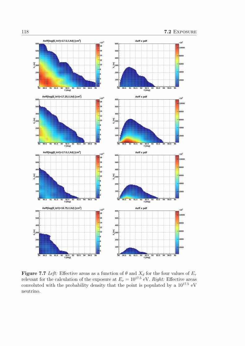
118 7.2 Exposure
[deg]θ90 90.5 91 91.5 92 92.5 93 93.5 94 94.5 95
[m
]d
X
0
100
200
300
400
500
600
2
4
6
8
10
12
14
16
18
1210×]2,Xd) [cmθ/eV)=17.5,τAeff(log(E
[deg]θ90 90.5 91 91.5 92 92.5 93 93.5 94 94.5 95
[m
]d
X
0
100
200
300
400
500
600
2000
4000
6000
8000
10000
310×Aeff x pdf
[deg]θ90 90.5 91 91.5 92 92.5 93 93.5 94 94.5 95
[m
]d
X
0
100
200
300
400
500
600
2
4
6
8
10
12
14
16
18
1210×]2,Xd) [cmθ/eV)=17.25,τAeff(log(E
[deg]θ90 90.5 91 91.5 92 92.5 93 93.5 94 94.5 95
[m
]d
X
0
100
200
300
400
500
600
2000
4000
6000
8000
10000
310×Aeff x pdf
[deg]θ90 90.5 91 91.5 92 92.5 93 93.5 94 94.5 95
[m
]d
X
0
100
200
300
400
500
600
2
4
6
8
10
12
14
16
18
1210×]2,Xd) [cmθ/eV)=17.0,τAeff(log(E
[deg]θ90 90.5 91 91.5 92 92.5 93 93.5 94 94.5 95
[m
]d
X
0
100
200
300
400
500
600
2000
4000
6000
8000
10000
310×Aeff x pdf
[deg]θ90 90.5 91 91.5 92 92.5 93 93.5 94 94.5 95
[m
]d
X
0
100
200
300
400
500
600
2
4
6
8
10
12
14
16
18
1210×]2,Xd) [cmθ/eV)=16.75,τAeff(log(E
[deg]θ90 90.5 91 91.5 92 92.5 93 93.5 94 94.5 95
[m
]d
X
0
100
200
300
400
500
600
2000
4000
6000
8000
10000
310×Aeff x pdf
Figure 7.7 Left: Effective areas as a function of θ and Xd for the four values of Eτ
relevant for the calculation of the exposure at Eν = 1017.5 eV. Right: Effective areasconvoluted with the probability density that the point is populated by a 1017.5 eVneutrino.
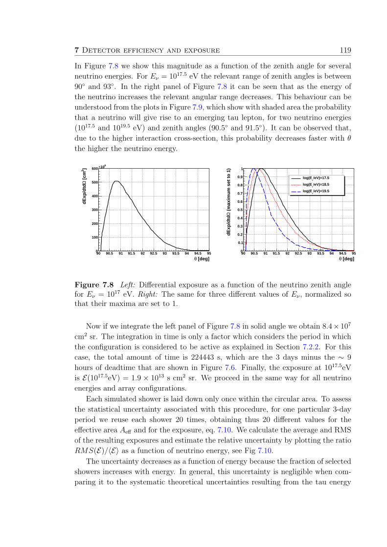
7 Detector efficiency and exposure 119
In Figure 7.8 we show this magnitude as a function of the zenith angle for several
neutrino energies. For Eν = 1017.5 eV the relevant range of zenith angles is between
90 and 93. In the right panel of Figure 7.8 it can be seen that as the energy of
the neutrino increases the relevant angular range decreases. This behaviour can be
understood from the plots in Figure 7.9, which show with shaded area the probability
that a neutrino will give rise to an emerging tau lepton, for two neutrino energies
(1017.5 and 1019.5 eV) and zenith angles (90.5 and 91.5). It can be observed that,
due to the higher interaction cross-section, this probability decreases faster with θ
the higher the neutrino energy.
[deg]θ90 90.5 91 91.5 92 92.5 93 93.5 94 94.5 95
]2 [
cmΩ
dE
xp/d
td
0
100
200
300
400
500
600610×
[deg]θ90 90.5 91 91.5 92 92.5 93 93.5 94 94.5 95
(m
axim
um
set
to
1)
Ωd
Exp
/dtd
0
0.1
0.2
0.3
0.4
0.5
0.6
0.7
0.8
0.9
1
/eV)=17.5ν
log(E
/eV)=18.5ν
log(E
/eV)=19.5ν
log(E
Figure 7.8 Left: Differential exposure as a function of the neutrino zenith anglefor Eν = 1017 eV. Right: The same for three different values of Eν , normalized sothat their maxima are set to 1.
Now if we integrate the left panel of Figure 7.8 in solid angle we obtain 8.4× 10⁷
cm2 sr. The integration in time is only a factor which considers the period in which
the configuration is considered to be active as explained in Section 7.2.2. For this
case, the total amount of time is 224443 s, which are the 3 days minus the ∼ 9
hours of deadtime that are shown in Figure 7.6. Finally, the exposure at 1017.5eV
is E(1017.5eV) = 1.9 × 10¹³ s cm2 sr. We proceed in the same way for all neutrino
energies and array configurations.
Each simulated shower is laid down only once within the circular area. To assess
the statistical uncertainty associated with this procedure, for one particular 3-day
period we reuse each shower 20 times, obtaining thus 20 different values for the
effective area Aeff and for the exposure, eq. 7.10. We calculate the average and RMS
of the resulting exposures and estimate the relative uncertainty by plotting the ratio
RMS(E)/〈E〉 as a function of neutrino energy, see Fig 7.10.
The uncertainty decreases as a function of energy because the fraction of selected
showers increases with energy. In general, this uncertainty is negligible when com-
paring it to the systematic theoretical uncertainties resulting from the tau energy
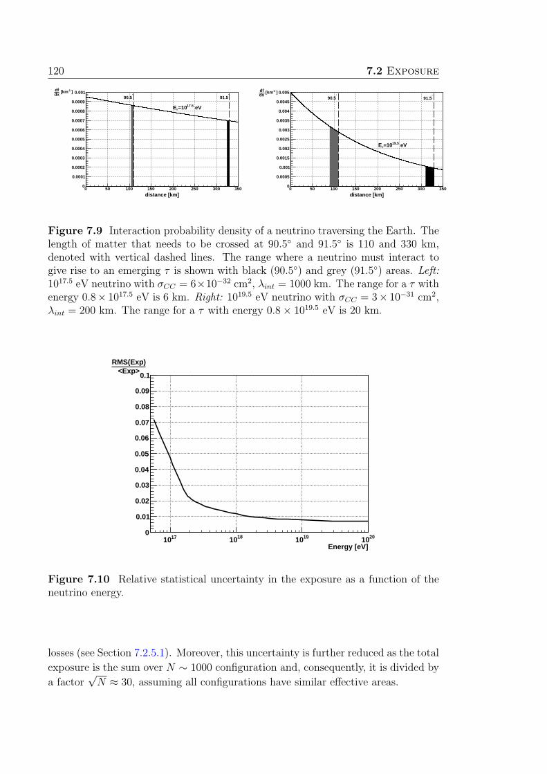
120 7.2 Exposure
distance [km]0 50 100 150 200 250 300 350
0
0.0001
0.0002
0.0003
0.0004
0.0005
0.0006
0.0007
0.0008
0.0009
0.001 ]-1 [kmdxdf
eV17.5=10νE
°90.5
°91.5
distance [km]0 50 100 150 200 250 300 350
0
0.0005
0.001
0.0015
0.002
0.0025
0.003
0.0035
0.004
0.0045
0.005 ]-1 [kmdxdf
eV19.5=10νE
°90.5
°91.5
Figure 7.9 Interaction probability density of a neutrino traversing the Earth. Thelength of matter that needs to be crossed at 90.5 and 91.5 is 110 and 330 km,denoted with vertical dashed lines. The range where a neutrino must interact togive rise to an emerging τ is shown with black (90.5) and grey (91.5) areas. Left:1017.5 eV neutrino with σCC = 6×10⁻³² cm2, λint = 1000 km. The range for a τ withenergy 0.8× 1017.5 eV is 6 km. Right: 1019.5 eV neutrino with σCC = 3× 10⁻³¹ cm2,λint = 200 km. The range for a τ with energy 0.8× 1019.5 eV is 20 km.
Energy [eV]1710 1810 1910 2010
0
0.01
0.02
0.03
0.04
0.05
0.06
0.07
0.08
0.09
0.1<Exp>
RMS(Exp)
Figure 7.10 Relative statistical uncertainty in the exposure as a function of theneutrino energy.
losses (see Section 7.2.5.1). Moreover, this uncertainty is further reduced as the total
exposure is the sum over N ∼ 1000 configuration and, consequently, it is divided by
a factor√N ≈ 30, assuming all configurations have similar effective areas.

7 Detector efficiency and exposure 121
7.2.4 Exposure results
In the previous section we explained the procedure to calculate the exposure. In
this section we present the results obtained.
In Chapter 6 we explained that there are two different selections applied to the
data. The first one is applied until May 20102, while the second one is applied from
June 2010 to December 2012. In Figure 7.11 we show the exposure for equal periods
of time for the case of the new and old criteria together with their ratio.
Energy [eV]1710 1810 1910 2010
s s
r]2
Exp
osu
re [
cm
1510
1610
1710
Old criteria
New criteria
Energy [eV]1710 1810 1910 2010
New
/Old
0.6
0.65
0.7
0.75
0.8
0.85
0.9
0.95
1
Figure 7.11 Top: Exposure of the SD corresponding to 1 year of a complete arraywhen applying the old and new criteria. Bottom: Ratio between the new and oldcriteria.
As expected the new criteria are less efficient than the old ones, a price to pay
for the stricter control of the background. The most important reason is that in
the new analysis 3-station events are only selected if they belong to configuration 1
(see Section 5.3.2). This is why the difference is largest towards lower neutrino
2Excluding November and December 2004.
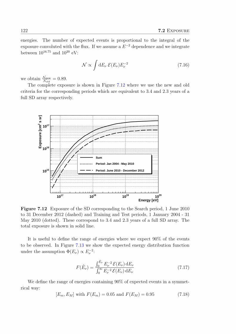
122 7.2 Exposure
energies. The number of expected events is proportional to the integral of the
exposure convoluted with the flux. If we assume a E−2 dependence and we integrate
between 1016.75 and 1020 eV:
N ∝∫
dEν E(Eν)E−2ν (7.16)
we obtain Nnew
Nold= 0.89.
The complete exposure is shown in Figure 7.12 where we use the new and old
criteria for the corresponding periods which are equivalent to 3.4 and 2.3 years of a
full SD array respectively.
Energy [eV]1710 1810 1910 2010
s s
r]2
Exp
osu
re [
cm
1510
1610
1710
Sum
Period: Jan 2004 - May 2010
Period: June 2010 - December 2012
Figure 7.12 Exposure of the SD corresponding to the Search period, 1 June 2010to 31 December 2012 (dashed) and Training and Test periods, 1 January 2004 - 31May 2010 (dotted). These correspond to 3.4 and 2.3 years of a full SD array. Thetotal exposure is shown in solid line.
It is useful to define the range of energies where we expect 90% of the events
to be observed. In Figure 7.13 we show the expected energy distribution function
under the assumption Φ(Eν) ∝ E−2ν :
F (Eν) =
∫ Eν
0E−2
ν E(Eν) dEν∫∞
0E−2
ν E(Eν) dEν
(7.17)
We define the range of energies containing 90% of expected events in a symmet-
rical way:
[Em, EM ] with F (Em) = 0.05 and F (EM) = 0.95 (7.18)

7 Detector efficiency and exposure 123
Energy [eV]1710 1810 1910 2010
) νF
(E
0
0.1
0.2
0.3
0.4
0.5
0.6
0.7
0.8
0.9
1
Figure 7.13 Expected energy distribution function F (Eν) under the assumptionof a flux with an energy dependence of E−2
ν . In dashed we show the region whichconcentrates 90% of the expected events: [1017, 1019.1] eV.
7.2.5 Systematic Uncertainties
The exposure calculation involves several factors. Some of them, such as the
cross-section, the tau energy loss and the hadronic model, are not known with
precision as they involve the extrapolation of measurements to uncharted kinematic
regions. In this context, it is useful to classify the choices made in the exposure
calculation into the following categories, as done in Chapter 4:
❼ Interactions in the Earth
❼ Interactions in the atmosphere
The purpose of this section is to describe the strategies used to estimate the
uncertainty associated to these two groups and discuss the final result.
7.2.5.1 Interactions in the Earth
The probability density functions f(Eτ |θ, Eν) used in the calculation of the expo-
sure (see equation 7.11) depend on the adopted parametrizations for the cross-section
and tau energy losses. A higher (lower) cross section for the neutrino charged in-
teraction ντ + N → τ + X (σCC) increases (decreases) the expected tau yield, so
we refer to them as the optimistic (pessimistic) case. On the other hand, a higher
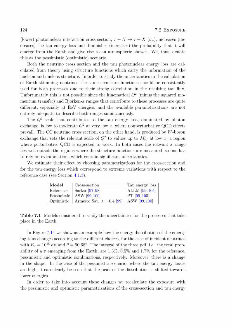
124 7.2 Exposure
(lower) photonuclear interaction cross section, τ +N → τ +X (σγ), increases (de-
creases) the tau energy loss and diminishes (increases) the probability that it will
emerge from the Earth and give rise to an atmospheric shower. We, thus, denote
this as the pessimistic (optimistic) scenario.
Both the neutrino cross section and the tau photonuclear energy loss are cal-
culated from theory using structure functions which carry the information of the
nucleon and nucleus structure. In order to study the uncertainties in the calculation
of Earth-skimming neutrinos the same structure functions should be consistently
used for both processes due to their strong correlation in the resulting tau flux.
Unfortunately this is not possible since the kinematical Q2 (minus the squared mo-
mentum transfer) and Bjorken-x ranges that contribute to these processes are quite
different, especially at EeV energies, and the available parametrizations are not
entirely adequate to describe both ranges simultaneously.
The Q2 scale that contributes to the tau energy loss, dominated by photon
exchange, is low to moderate Q2 at very low x, where nonperturbative QCD effects
prevail. The CC neutrino cross section, on the other hand, is produced by W -boson
exchange that sets the relevant scale of Q2 to values up to M2W at low x, a region
where perturbative QCD is expected to work. In both cases the relevant x range
lies well outside the regions where the structure functions are measured, so one has
to rely on extrapolations which contain significant uncertainties.
We estimate their effect by choosing parametrizations for the cross-section and
for the tau energy loss which correspond to extreme variations with respect to the
reference case (see Section 4.1.3).
Model Cross-section Tau energy loss
Reference Sarkar [97, 98] ALLM [99,104]Pessimistic ASW [99,100] PT [99,105]Optimistic Armesto Sat. λ = 0.4 [99] ASW [99,100]
Table 7.1 Models considered to study the uncertainties for the processes that takeplace in the Earth.
In Figure 7.14 we show as an example how the energy distribution of the emerg-
ing taus changes according to the different choices, for the case of incident neutrinos
with Eν = 1018 eV and θ = 90.68. The integral of the three pdf, i.e. the total prob-
ability of a τ emerging from the Earth, are 1.3%, 0.5% and 1.7% for the reference,
pessimistic and optimistic combinations, respectively. Moreover, there is a change
in the shape. In the case of the pessimistic scenario, where the tau energy losses
are high, it can clearly be seen that the peak of the distribution is shifted towards
lower energies.
In order to take into account these changes we recalculate the exposure with
the pessimistic and optimistic parametrizations of the cross-section and tau energy

7 Detector efficiency and exposure 125
16 16.2 16.4 16.6 16.8 17 17.2 17.4 17.6 17.8 180
0.002
0.004
0.006
0.008
0.01
0.012
0.014
0.016
0.018
0.02
0.022
)τ(E10
dlogτdn
/eV)τ(E10
log
Reference - Sarkar - ALLM
Pesimistic: ASW - PT
=0.4 - ASWλOptimistic - Armesto Sat
Figure 7.14 Energy probability density for an emerging tau. The function dependson the parametrizations of the cross-section and tau energy loss. In this examplethe energy is fixed at Eν = 1018 eV and the zenith angle at θ = 90.68.
losses. The result is shown in Figure 7.15 where it can be seen that the optimistic
scenario is higher than the reference by ∼15% at the lowest energies and it reaches a
maximum of ∼50% at 1019 eV. On the other hand, the pessimistic scenario is lower
by -45% at the lowest energies and it reaches -70% at 1018 eV. A calculation of the
average differences weighted with a E−2 flux factor over the region where we expect
90% of the events yields a [−65%,+37%].
In Figure 7.15 we also show the relative differences changing separately the cross-
section or the tau energy losses. It is clear that tau energy losses are dominant over
the entire energy range.
The dependence of the exposure on the neutrino cross section decreases due
to the competition between two effects: the tau yield over the complete distance
travelled through the Earth increases with the cross-section, while the fraction of τs
produced in the range where they can emerge to the surface decreases.
7.2.5.2 Interactions in the atmosphere
The simulation of MC events initiated by a τ lepton involves two sources of
systematic uncertainty:
1. The hadronic interaction model at high energy (QGSJETII).
2. The atmospheric shower evolution (AIRES 2.8 with a relative thinning of
10−6).
where the actual option chosen to generate the MC sample of showers induced by
a τ decay is indicated in parenthesis. To estimate the systematic uncertainty, we
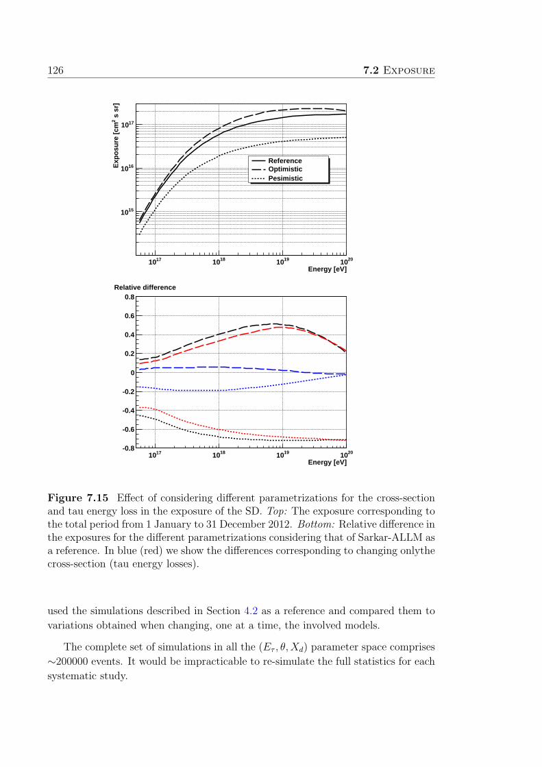
126 7.2 Exposure
Energy [eV]1710 1810 1910 2010
s s
r]2
Exp
osu
re [
cm
1510
1610
1710
ReferenceOptimisticPesimistic
Energy [eV]1710 1810 1910 2010
-0.8
-0.6
-0.4
-0.2
0
0.2
0.4
0.6
0.8Relative difference
Figure 7.15 Effect of considering different parametrizations for the cross-sectionand tau energy loss in the exposure of the SD. Top: The exposure corresponding tothe total period from 1 January to 31 December 2012. Bottom: Relative difference inthe exposures for the different parametrizations considering that of Sarkar-ALLM asa reference. In blue (red) we show the differences corresponding to changing onlythecross-section (tau energy losses).
used the simulations described in Section 4.2 as a reference and compared them to
variations obtained when changing, one at a time, the involved models.
The complete set of simulations in all the (Eτ , θ,Xd) parameter space comprises
∼200000 events. It would be impracticable to re-simulate the full statistics for each
systematic study.

7 Detector efficiency and exposure 127
The alternative is to select only a representative fraction of the parameter space.
Accordingly, we chose 20 points having a high value of the weight, as defined in
Section 4.3, Eq. 4.18. These 20 points are shown in Figure 7.16 and represent ∼30%
of the total weight.
logE/eV16.5 17 17.5 18
[deg]
θ
8788
8990
X [
m]
0
100
200
300
400
500
600
700
800
900
1000
Figure 7.16 In black the points in the parameter space log10Eτ
eV, θ and decay
height Xd, that have been simulated in the range [16.5, 18], [90, 93] and [0, 1000m]respectively. In red the selected points with high weight value selected to study thesystematic uncertainties due to the interactions in the atmosphere.
The magnitude used to perform a comparison between the different models is
the sum of the weights (∑
i wi, see Section 4.3) over the selected and identified
showers, which is proportional to the number of expected events. In Table 7.2
we summarize the results. The differences obtained provide an estimation of the
uncertainty between the selected models. It can be observed that the differences
are small when compared to the statistical uncertainty (∼5%). This means that the
systematics associated to the hadronic model or the thinning factor can be neglected.
Parameter Reference Modification Difference
(A) (B) B−A
(B+A)/2
Hadronic model QGSJETII QGSJETI [110] +4.7%SIBYLL [109] -1.0%
Thinning 10−6 10−7 +0.3%
Table 7.2 Summary of the relative differences between alternative models involvedin the shower simulation. The statistical uncertainty in the relative differences is∼5%.

128 7.2 Exposure
In summary, the uncertaities in the interaction in the Earth dominate over the
uncertainties of the simulation of the shower. In particular, the most important
effect comes from the tau energy loss models.
8Results and discussion
As described in Chapter 6, this work used a blind search scheme. The data anal-
ysed was divided into three groups: the first two, training and test samples, were
used to characterize the detector and develop an algorithm for neutrino identifica-
tion. The third, search sample, was not scanned until after defining the identification
criteria. The procedure of applying the neutrino identification criteria to the events
in the search sample is denominated colloquially as “opening the box”
In this Chapter we first apply the identification criteria to the Search sample
(Section 8.1). In Sections 8.3 and 8.4 we analyze the number of expected neutrino
events under different diffuse neutrino flux predictions and place a limit on the
normalization of a flux with a E−2 dependence. Finally, in Section 8.5, we study
the case of a high energy neutrino flux from a specific point in the sky (point-like
sources) and place limits which are dependent on the declination of the source.
8.1 Blind search: “opening the box”
Once the identification criteria is defined, the next step is to analyse the search
sample (1 June 2010 - 31 December 2012) applying the following steps:
1. Selection of quality events
2. Selection of inclined events
3. Calculation of the 〈AoP〉 for each event
4. Selection of events with 〈AoP〉 > 〈AoP〉cut = 1.82
5. For 3-station events, demand AoP min > 1.4.
129

130 8.1 Blind search: “opening the box”
There are 0 candidates after applying these criteria. In Figure 8.1 we present the
distribution of 〈AoP〉 for the events in the search sample. The number of expected
events according to the background distributions predicted from the Test sample
(see Section 6.6) and the number of actually measured events in the Search sample
are compared in the four testing regions ([3σ, 4σ], [4σ, 5σ], [5σ, 6σ] and [6σ, 7σ]).
There is agreement between measurements and predictions in all the regions within
the poissonian statistical fluctuations.
Figure 8.1 Distribution of 〈AoP〉 of the data events in the Search sample (1June 2010 - 31 December 2012). The regions [3σ, 4σ], [4σ, 5σ], [5σ, 6σ] and [6σ, 7σ]are defined by the Test sample and are shown between dashed vertical lines (seeSection 6.6). The predicted number of events for each region according to theexponential fit to the Test sample (Pred.) are in agreement with the number ofmeasured events in the Search sample (Real).
We have also seen in Section 6.6.1 that there was an evolution of the calibrated
value of area over peak from the Training sample to the Test sample. In Figure 8.2
we show the evolution with time of the mean value of the distribution of 〈AoP〉including now the Search sample.
The rise in the average calibrated area over peak (〈AoP〉cal) seems to stop within
the statistical uncertainties considered. The effect could be related to the observa-
tion that the uncalibrated vertical muon area over peak (AoPunc) of single stations
decreased with time by around 10% over the first years of data taking and then it
stabelized [126]. This is the opposite pattern of Figure 8.2, which could result from
an overcorrection for inclined muons due to the station area and peak calibration
derived with vertical muons. Further studies need to be taken however to under-

8 Results and discussion 131
month0 20 40 60 80 100
<Ao
P>
1.14
1.15
1.16
1.17
1.18
1.19
1.2
1.21
1.22
Figure 8.2 Mean value of the distribution of 〈AoP〉 per month, from January 2004(month 0) to December 2012 (month 108). In black (red/blue) dots we show themonths corresponding to the Training (Test/Search) sample.
stand this effect which is beyond the scope of this dissertation. We emphasize that
this effect is nevertheless negligible for the estimation of the expected number of
background events, as discussed in Section 6.6.2.
8.2 Comparison to theory: statistical treatment
In order to define the number of expected events necessary to reject a flux model
with 90% confidence level (CL) it is instructive to consider first a simplified case
in which we assume a negligible background and an exposure with no uncertainty.
The number of observed events n is a random variable with a Poissonian distribution
Pα(n), where α is the expected number of events. For a given theoretical prediction
we refer to α as Nsignal, which is calculated as:
Nsignal =
∫ Emax
Emin
Φ(Eν) E(Eν) dEν (8.1)
where Φ(Eν) is the neutrino diffuse flux under consideration, E(Eν) is the exposure
of the detector and [Emin, Emax] is the energy range.
If α is known, the probability of observing at least one neutrino is given by:
Pα(n ≥ 1) = 1−Pα(0). Inversely, knowing that the experiment observed no neutrino,
the estimated confidence region of α with p× 100% CL is defined as Pα(n ≥ 1) < p.
This confidence region is [0, α], where the estimator for the the upper limit, α, is

132 8.2 Comparison to theory: statistical treatment
obtained from:
Pα(n ≥ 1) = p ⇒ 1− Pα(0) = p ⇒ Pα(0) = 1− p (8.2)
In particular, the upper limit with a 90% CL is:
1− Pα(0) = 0.9 ⇒ 1− e−α = 0.9 ⇒ α ≃ 2.3 ⇒ 0 < α < 2.3 (8.3)
This simplified approach, presented only for pedagical reasons, presents essen-
tially three shortcomings:
1. It does not allow for the possible presence of a background contribution to the
number of observed events
2. It only applies for upper bounds, rather than offering a unified treatment that
can also yield a range for alpha, with lower and upper limits, depending on
the number of observed events.
3. It does not consider the contribution of systematic uncertainties to the esti-
mator α.
The first two points were addressed by Feldman and Cousins (FC) [127], who pro-
posed an unified approach for the classical statistical analysis of small signals based
on the confidence belt frequentist construction and the likelihood ratio ordering
method. Given a number of observed events, and a predicted background, the FC
approach univocally produces upper bounds or confidence ranges. For the particular
case of a background free experiment with no events observed, the FC prescription
amounts to replace the factor 2.3 by 2.44 in equation 8.3:
αpoisson ≃ 2.3 ⇒ αFC = 2.44 ⇒ 0 < α < 2.44 (8.4)
Although this scheme provides a unified framework to calculate the limits (up-
per and lower) with background, it does not include the treatment of systematic
uncertainties. Conrad et al developed in [128] a semi bayesian extension of the
method which incorporates the systematic contributions to the exposure E(Eν) and
the background estimation, Nbkg. The fixed values of E(Eν) andNbkg are replaced by
probability density functions (pdf) f(E) and f(Nbkg) which quantify our knowledge
of their possible values.
Then, before applying this method it is necessary to establish the probabil-
ity density functions which characterize the number of expected events Nsignal and
Nbkg. The pdf of Nsignal is determined by the uncertainty on the total exposure.
As discussed in Section 7.2.5.1, the uncertainty is [-65%, +37%] and we assume a
uniform distribution for it.

8 Results and discussion 133
In order to estimate Nbkg we recall that in Chapter 6 the neutrino identification
criterion, 〈AoP〉 > 1.82, was defined so that there is one expected background event
in 50 years. As the Search period corresponds to 2.3 years of a fully deployed SD
the actual expected background is ∼ 2.350
= 0.046. The distribution of background is
obtained from the linear extrapolation in log scale:
N2.3yrbkg (〈AoP〉) = 2.3
2.0eA−B〈AoP〉 (8.5)
where A and B are obtained from the fit to the Test sample, which corresponds to
2 years of a fully deployed SD. Under the assumption of binormal distribution of
A and B, using the covariance matrix from the fit, we obtain a probability density
function for the number of background events:
Nbkg =1
∆〈AoP〉
∫ ∞
1.82
d〈AoP〉 N2.3yr(〈AoP〉) = 1
∆〈AoP〉2.3
2.0
eA−B×1.82
B(8.6)
which is shown in Figure 8.3.
BkgN0 0.05 0.1 0.15 0.2 0.25 0.3
Bkg
dNd
p
0
2
4
6
8
10
12
14
16
18
20
68% CL Interval
Figure 8.3 Probability density function of expected number of background events.
It has to be noticed that the period unblinded under the Old ES criteria has
claimed 0 background events. Consequently, the 68% CL background expectation
for the total period is [0.02, 0.1], as shown in Figure 8.3.
Given that the estimated background is small and that it suffers from unknown
systematic uncertainties, the number of background events will be assumed to be
0, which results in a more conservative (higher) α. Using the background free
assumption but including the systematic uncertainties on the exposure, we obtain
134 8.3 Testing theoretical predictions
that the 90% CL region for the number of expected events is:
αConrad = 3.21 ⇒ 0 < α < 3.21 (8.7)
This means that, for the case of zero observed events, the number of expected
events should be greater than 3.21 to reject a given neutrino flux model. The
increase on α is the direct consequence of including the systematic uncertainties on
the exposure which are asymmetrical and larger towards lower values. It is worth
noticing that the method is not very sensitive to the choice of the functional form
of the distributions of E or Nbkg. Moreover, if we included the effect of the small
background estimated in Figure 8.3 αConrad would be reduced from 3.21 to 3.13,
which is negligible.
8.3 Testing theoretical predictions
As discussed in Chapter 1 there is large number of theoretical models predicting
neutrino fluxes with energies around 1 EeV. Using the exposure E(Eν) accumulated
by the Pierre Auger Collaboration from 1 January 2004 to 31 December 2012 the
expected number of events, Nsignal, for a diffuse neutrino flux Φ(Eν) can be obtained
by integrating in energy as in equation 8.1.
The integration can be performed over the entire range of energy or in bins to
analyse where the sensitivity of the detector is highest. It needs to be mentioned that
Φ(Eν) is the flux of ντ , so in case Φ(Eν) corresponds to an all flavour flux, it needs
to be divided by 3 under the assumption of the 1:1:1 ratio expected from neutrino
oscillations over cosmological distances. In Figure 8.4 we show the expected number
of events for the GZK-FermiLat flux prediction (presented in Section 1.2.1) as a
function of energy. It can be seen that the sensitivity peaks at 1018 eV. This is to
be expected as at high energy the flux decrease overcomes the rise in the exposure,
while at energies below 1018 eV the lower exposure overcomes the higher flux. This
behaviour applies to all models where the flux, to first order, behaves with energy
as E−2.
The expected signal from GZK-FermiLat diffuse flux of UHE neutrinos is 1.8+0.8−1.2.
The signal to background ratio is 18 considering the upper limit of the 68% CL
interval for the background. This means that for this flux we are not limited by the
background.
In Table 8.1 we summarize the results for the set of selected models presented in
Section 1.2. We also estimate the additional data taking time needed to reject the
model at 90% CL, under the assumption that no event is observed.
The most reliable prediction of existence of diffuse neutrinos corresponds to
those of cosmogenic origin. As it can be seen there are a variety of models which
predict the observation of ∼1 event within the present accumulated statistics. If
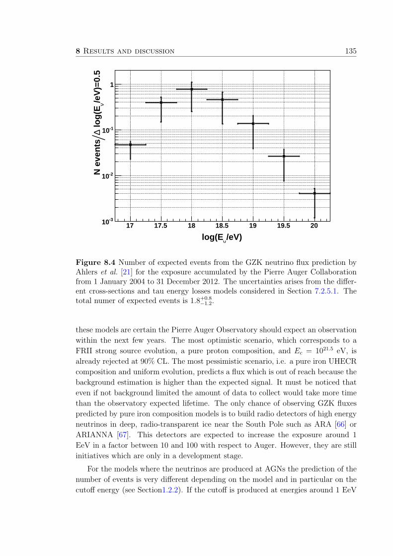
8 Results and discussion 135
/eV)ν
log(E17 17.5 18 18.5 19 19.5 20
/eV
)=0.
5ν
log
(E∆
N e
ven
ts
-310
-210
-110
1
Figure 8.4 Number of expected events from the GZK neutrino flux prediction byAhlers et al. [21] for the exposure accumulated by the Pierre Auger Collaborationfrom 1 January 2004 to 31 December 2012. The uncertainties arises from the differ-ent cross-sections and tau energy losses models considered in Section 7.2.5.1. Thetotal numer of expected events is 1.8+0.8
−1.2.
these models are certain the Pierre Auger Observatory should expect an observation
within the next few years. The most optimistic scenario, which corresponds to a
FRII strong source evolution, a pure proton composition, and Ec = 1021.5 eV, is
already rejected at 90% CL. The most pessimistic scenario, i.e. a pure iron UHECR
composition and uniform evolution, predicts a flux which is out of reach because the
background estimation is higher than the expected signal. It must be noticed that
even if not background limited the amount of data to collect would take more time
than the observatory expected lifetime. The only chance of observing GZK fluxes
predicted by pure iron composition models is to build radio detectors of high energy
neutrinos in deep, radio-transparent ice near the South Pole such as ARA [66] or
ARIANNA [67]. This detectors are expected to increase the exposure around 1
EeV in a factor between 10 and 100 with respect to Auger. However, they are still
initiatives which are only in a development stage.
For the models where the neutrinos are produced at AGNs the prediction of the
number of events is very different depending on the model and in particular on the
cutoff energy (see Section1.2.2). If the cutoff is produced at energies around 1 EeV
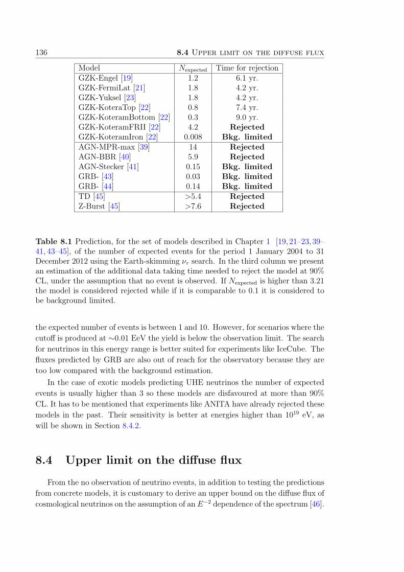
136 8.4 Upper limit on the diffuse flux
Model Nexpected Time for rejectionGZK-Engel [19] 1.2 6.1 yr.GZK-FermiLat [21] 1.8 4.2 yr.GZK-Yuksel [23] 1.8 4.2 yr.GZK-KoteraTop [22] 0.8 7.4 yr.GZK-KoteramBottom [22] 0.3 9.0 yr.GZK-KoteramFRII [22] 4.2 RejectedGZK-KoteramIron [22] 0.008 Bkg. limitedAGN-MPR-max [39] 14 RejectedAGN-BBR [40] 5.9 RejectedAGN-Stecker [41] 0.15 Bkg. limitedGRB- [43] 0.03 Bkg. limitedGRB- [44] 0.14 Bkg. limitedTD [45] >5.4 RejectedZ-Burst [45] >7.6 Rejected
Table 8.1 Prediction, for the set of models described in Chapter 1 [19, 21–23, 39–41, 43–45], of the number of expected events for the period 1 January 2004 to 31December 2012 using the Earth-skimming ντ search. In the third column we presentan estimation of the additional data taking time needed to reject the model at 90%CL, under the assumption that no event is observed. If Nexpected is higher than 3.21the model is considered rejected while if it is comparable to 0.1 it is considered tobe background limited.
the expected number of events is between 1 and 10. However, for scenarios where the
cutoff is produced at ∼0.01 EeV the yield is below the observation limit. The search
for neutrinos in this energy range is better suited for experiments like IceCube. The
fluxes predicted by GRB are also out of reach for the observatory because they are
too low compared with the background estimation.
In the case of exotic models predicting UHE neutrinos the number of expected
events is usually higher than 3 so these models are disfavoured at more than 90%
CL. It has to be mentioned that experiments like ANITA have already rejected these
models in the past. Their sensitivity is better at energies higher than 1019 eV, as
will be shown in Section 8.4.2.
8.4 Upper limit on the diffuse flux
From the no observation of neutrino events, in addition to testing the predictions
from concrete models, it is customary to derive an upper bound on the diffuse flux of
cosmological neutrinos on the assumption of an E−2 dependence of the spectrum [46].
8 Results and discussion 137
8.4.1 Integral limit
If for the three neutrino flavours a typical differential flux with an energy depen-
dence of Φνx = kνx · E−2ν is chosen, the result is:
N totalsignal = N νe
signal +Nνµsignal +N ντ
signal (8.8)
where each of the N νxsignal is:
N νxsignal = kνx
∫ Emax
Emin
E−2ν EνX(Eν) dEν
︸ ︷︷ ︸
≡N (Eνx )
= kνx · N (Eνx) (8.9)
The magnitude N (E) has units of [GeV−1 cm2 s sr] and depends only on the
exposure E . The integration is performed in the energy interval [1017, 1019.1] eV that
contains 90% of expected events, see Section 7.2.4. This is the standard definition
of the upper limit. If a 1:1:1 ratio between flavours is assumed:
kνe = kνµ = kντ ≡ kSF =kAll
3(8.10)
where kSF is the normalization of a single flavour flux, equation 8.8 can be expressed
in a more compact way:
N totalsignal = kSF · (N νe +N νµ +N ντ ) = kSF · N total =
kAll
3· N total (8.11)
This expression allows us to obtain a limit over the magnitude of the total neu-
trino flux kAll 1. If we consider the Feldman-Cousins approach in which we assume
negligible background and no systematic uncertainty as it has been discussed in
Section 8.2 an upper limit on kAll with 90% CL is set by:
N totalsignal =
kAll
3· N total
N totalsignal ≤ 2.44
=⇒ kAll
3≤ 2.44
N total(8.12)
If one uses the total exposure for the period 1 January 2004 to 31 December
2012, the result is:
kAll ≤ 3.8× 10⁻⁸ GeV cm−2 s−1 sr−1 (8.13)
over the energy range from 1017 eV to 1019.1 eV.
Including systematic uncertainties discussed in Section 8.2 with N totalsignal ≤ 3.21
1The limit over the magnitude of the single flavour neutrino flux is obtained dividing kAll by 3.
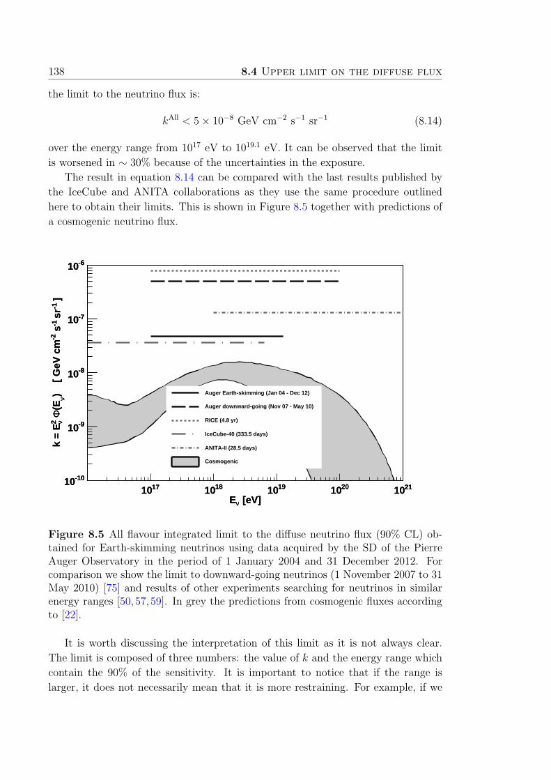
138 8.4 Upper limit on the diffuse flux
the limit to the neutrino flux is:
kAll < 5× 10⁻⁸ GeV cm−2 s−1 sr−1 (8.14)
over the energy range from 1017 eV to 1019.1 eV. It can be observed that the limit
is worsened in ∼ 30% because of the uncertainties in the exposure.
The result in equation 8.14 can be compared with the last results published by
the IceCube and ANITA collaborations as they use the same procedure outlined
here to obtain their limits. This is shown in Figure 8.5 together with predictions of
a cosmogenic neutrino flux.
[eV]νE1710 1810 1910 2010 2110
]-1
sr
-1 s
-2)
[
GeV
cm
ν(E
Φ ν2k
= E
-1010
-910
-810
-710
-610
[eV]νE1710 1810 1910 2010 2110
]-1
sr
-1 s
-2)
[
GeV
cm
ν(E
Φ ν2k
= E
-1010
-910
-810
-710
-610
Auger Earth-skimming (Jan 04 - Dec 12)
Auger downward-going (Nov 07 - May 10)
RICE (4.8 yr)
IceCube-40 (333.5 days)
ANITA-II (28.5 days)
Cosmogenic
Figure 8.5 All flavour integrated limit to the diffuse neutrino flux (90% CL) ob-tained for Earth-skimming neutrinos using data acquired by the SD of the PierreAuger Observatory in the period of 1 January 2004 and 31 December 2012. Forcomparison we show the limit to downward-going neutrinos (1 November 2007 to 31May 2010) [75] and results of other experiments searching for neutrinos in similarenergy ranges [50, 57, 59]. In grey the predictions from cosmogenic fluxes accordingto [22].
It is worth discussing the interpretation of this limit as it is not always clear.
The limit is composed of three numbers: the value of k and the energy range which
contain the 90% of the sensitivity. It is important to notice that if the range is
larger, it does not necessarily mean that it is more restraining. For example, if we
8 Results and discussion 139
consider two limits with the same k but the second one covers twice the range than
the first one, this means that the first limit is twice more stringent than the second
in the range of energies where they overlap. This is simply because the second limit
needs to integrate over a larger range of energies to obtain the same bound. This
is why, traditionally, the community not only compares integrated limits but also
quasi-differential limits which are useful to quantify the sensitivity region of each
experiment. Quasi-differential limits are explained in the following section.
8.4.2 Quasi-differential limit
In the calculation of the integrated limit it was necessary to assume that the
neutrino flux depends on the energy like Φ(Eν) = k E−2, with constant k in the
energy range from 1017 to 1019.1 eV. This hypotesis, although reasonable, can be
incorrect and it is interesting to study the effect of replacing it with a less restrictive
option: considering that the intensity of the flux k has a small dependence on
the energy and, consequently, the approximation of the energy dependence E−2 is
appropiate in small energy ranges.
In this way, around a defined energy E there is a range in which the flux can be
approximated by k(E)E−2 with k(E) constant so that the integrated limit can be
calculated over a restricted range.
Including the systematic uncertainties by considering the factor 3.21, the upper
limit in a range ∆E(Eν) which depends on the energy can be written as:
k(Eν) ≤3.21
N (Eν)with N (Eν) =
∫
∆E(Eν)
E ′−2ν E(E ′
ν) dE′ν (8.15)
When choosing ∆E(Eν) such that all integration ranges have equal width in the
logarithmic scale, the result is:
k(Eν) ≤ 3.21/ 1
ln 10
∫ log10(Eν)+∆ log10(Eν)/2
log10(Eν)−∆ log10(Eν)/2
E ′−1ν E(E ′
ν) d(log10(E′ν)) (8.16)
This way of presenting the upper limit is commonly denoted “quasi-differential
limit”.
In Figure 8.6 the obtained differential limit is presented together with previous
results in a similar energy range. It is interesting to notice that the limits set by
the SD of the Pierre Auger Collaboration achieve maximum sensitivity in the same
energy region where the flux of cosmogenic neutrinos is expected to peak. It can
be seen that in the range of energies between 1017 and 1019 eV we place the most
stringent limits. However, it needs to be noted that in one of the most recent
publication of IceCube [51], where they present the first two PeV neutrinos, they
analyse data from twice the effective lifetime and twice the number of strings than
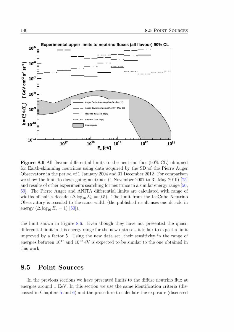
140 8.5 Point Sources
[eV]νE1710 1810 1910 2010 2110
]-1
sr
-1 s
-2)
[
GeV
cm
ν(E
Φ ν2k
= E
-1110
-1010
-910
-810
-710
-610
-510Experimental upper limits to neutrino fluxes (all flavour) 90% CL
[eV]νE1710 1810 1910 2010 2110
]-1
sr
-1 s
-2)
[
GeV
cm
ν(E
Φ ν2k
= E
-1110
-1010
-910
-810
-710
-610
-510
Auger Earth-skimming (Jan 04 - Dec 12)
Auger downward-going (Nov 07 - May 10)
IceCube-40 (333.5 days)
ANITA-II (28.5 days)
Cosmogenic
Figure 8.6 All flavour differential limits to the neutrino flux (90% CL) obtainedfor Earth-skimming neutrinos using data acquired by the SD of the Pierre AugerObservatory in the period of 1 January 2004 and 31 December 2012. For comparisonwe show the limit to down-going neutrinos (1 November 2007 to 31 May 2010) [75]and results of other experiments searching for neutrinos in a similar energy range [50,59]. The Pierre Auger and ANITA differential limits are calculated with range ofwidths of half a decade (∆ log10 Eν = 0.5). The limit from the IceCube NeutrinoObservatory is rescaled to the same width (the published result uses one decade inenergy (∆ log10 Eν = 1) [50]).
the limit shown in Figure 8.6. Even though they have not presented the quasi-
differential limit in this energy range for the new data set, it is fair to expect a limit
improved by a factor 5. Using the new data set, their sensitivity in the range of
energies between 1017 and 1019 eV is expected to be similar to the one obtained in
this work.
8.5 Point Sources
In the previous sections we have presented limits to the diffuse neutrino flux at
energies around 1 EeV. In this section we use the same identification criteria (dis-
cussed in Chapters 5 and 6) and the procedure to calculate the exposure (discussed
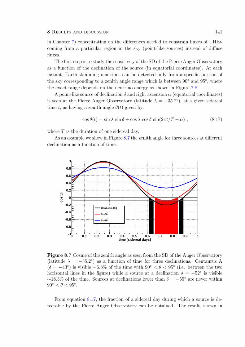
8 Results and discussion 141
in Chapter 7) concentrating on the differences needed to constrain fluxes of UHEν
coming from a particular region in the sky (point-like sources) instead of diffuse
fluxes.
The first step is to study the sensitivity of the SD of the Pierre Auger Observatory
as a function of the declination of the source (in equatorial coordinates). At each
instant, Earth-skimming neutrinos can be detected only from a specific portion of
the sky corresponding to a zenith angle range which is between 90 and 95, where
the exact range depends on the neutrino energy as shown in Figure 7.8.
A point-like source of declination δ and right ascension α (equatorial coordinates)
is seen at the Pierre Auger Observatory (latitude λ = −35.2), at a given sidereal
time t, as having a zenith angle θ(t) given by:
cos θ(t) = sinλ sin δ + cosλ cos δ sin(2πt/T − α) , (8.17)
where T is the duration of one sidereal day.
As an example we show in Figure 8.7 the zenith angle for three sources at different
declination as a function of time.
time [sidereal days]0 0.1 0.2 0.3 0.4 0.5 0.6 0.7 0.8 0.9 1
)θco
s(
-1
-0.8
-0.6
-0.4
-0.2
0
0.2
0.4
0.6
0.8
1
)°
=-43δCenA (
°=-50δ
°=-70δ
Figure 8.7 Cosine of the zenith angle as seen from the SD of the Auger Observatory(latitude λ = −35.2) as a function of time for three declinations. Centaurus A(δ = −43) is visible ∼6.8% of the time with 90 < θ < 95 (i.e. between the twohorizontal lines in the figure) while a source at a declination δ = −52 is visible∼18.3% of the time. Sources at declinations lower than δ = −55 are never within90 < θ < 95.
From equation 8.17, the fraction of a sidereal day during which a source is de-
tectable by the Pierre Auger Observatory can be obtained. The result, shown in
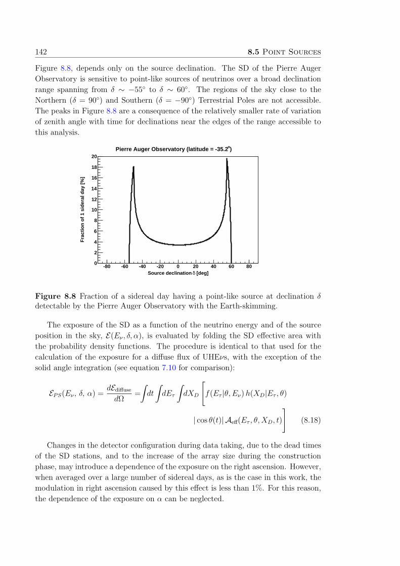
142 8.5 Point Sources
Figure 8.8, depends only on the source declination. The SD of the Pierre Auger
Observatory is sensitive to point-like sources of neutrinos over a broad declination
range spanning from δ ∼ −55 to δ ∼ 60. The regions of the sky close to the
Northern (δ = 90) and Southern (δ = −90) Terrestrial Poles are not accessible.
The peaks in Figure 8.8 are a consequence of the relatively smaller rate of variation
of zenith angle with time for declinations near the edges of the range accessible to
this analysis.
[deg]δSource declination -80 -60 -40 -20 0 20 40 60 80
Fra
ctio
n o
f 1
sid
eral
day
[%
]
0
2
4
6
8
10
12
14
16
18
20)oPierre Auger Observatory (latitude = -35.2
Figure 8.8 Fraction of a sidereal day having a point-like source at declination δdetectable by the Pierre Auger Observatory with the Earth-skimming.
The exposure of the SD as a function of the neutrino energy and of the source
position in the sky, E(Eν , δ, α), is evaluated by folding the SD effective area with
the probability density functions. The procedure is identical to that used for the
calculation of the exposure for a diffuse flux of UHEνs, with the exception of the
solid angle integration (see equation 7.10 for comparison):
EPS(Eν , δ, α) =dEdiffusedΩ
=
∫
dt
∫
dEτ
∫
dXD
[
f(Eτ |θ, Eν)h(XD|Eτ , θ)
| cos θ(t)| Aeff(Eτ , θ,XD, t)
]
(8.18)
Changes in the detector configuration during data taking, due to the dead times
of the SD stations, and to the increase of the array size during the construction
phase, may introduce a dependence of the exposure on the right ascension. However,
when averaged over a large number of sidereal days, as is the case in this work, the
modulation in right ascension caused by this effect is less than 1%. For this reason,
the dependence of the exposure on α can be neglected.

8 Results and discussion 143
The dependence of the exposure on the source declination comes through θ(t)
as obtained from equation 8.17. The integration over time, only considers those
periods when the source is within the zenith angle range of the neutrino selection.
The expected number of neutrino events in an energy range [Emin, Emax] detected
by the Pierre Auger Observatory from a point-like source located at a declination δ
is given by:
Npoint sourceexpected (δ) =
∫ Emax
Emin
F (Eν , δ) E(Eν , δ) dEν , (8.19)
where F (Eν , δ) is the differential flux of UHEνs from a source at a declination δ so
it is the intensity per unit of time, area and energy2.
We have already mentioned that no candidate events have been found. Assuming
a differential flux with an energy dependence of F (Eν , δ) = kPS(δ) ·E−2ν , a 90% C.L.
upper limit on the neutrino flux from point-like sources can be obtained following
the same considerations as in Section 8.4.
In Figure 8.9, the 90% C.L. upper limit on kPS is shown as a function of source
declination. Limits for kPS at the level of ≈ 8 × 10⁻⁷ GeV cm−2 s−1 are obtained
over a broad range of declinations considering Earth-skimming neutrinos.
Source declination [deg]-80 -60 -40 -20 0 20 40 60 80
]-1
s-2
F(E
) [G
eV c
m2
=EP
Sk
-710
-610
-510
All flavour neutrino limits (90% CL)
Auger Earth-skimming (Jan 04 - Dic 2012)
Auger donward-going (Nov 07 - May 2010)
Figure 8.9 Upper limits at 90% C.L. on an all flavour E−2ν flux from a specific
point-like source as a function of the source declination.
The shape of the declination-dependent upper limits is largely determined by
the fraction of time a source is within the field of view (see Figure 8.8), and, to a
lesser extent, by the zenith angle dependence of the exposure.
2The diffuse flux Φ(Eν) is the intensity per unit of time, area, energy and solid angle.

144 8.5 Point Sources
The upper limits are derived for neutrinos in the energy range 1017 eV−1019.1 eV,
with a negligible dependence of these energy intervals on the source declination. This
is the best limit in the literature around 1 EeV. The IceCube Neutrino Observatory
and the Antares Neutrino Telescope have also searched for UHEνs from point-like
sources ( [129] and [130], respectively). The bounds obtained by these two experi-
ments apply to energies below the Auger energy range.
Limits for the particular case of the active galaxy Centaurus A, a potential
source of UHECRs, are shown in Figure 8.10, together with constraints from other
experiments. The predicted fluxes for two theoretical models of UHEν production
in the jets [131] and close to the core [132] of Centaurus A are also shown for
comparison. The expected number of events for these models are 0.2 and 0.04
respectively, beyond the present reach of the experiment.
energy [eV]ν1510 1610 1710 1810 1910 2010 2110 2210 2310
]-1
s-2
F(E
) [G
eV c
m2
=EP
Sk
-910
-810
-710
-610
-510
-410
Centaurus A - All flavour neutrino limits (90% CL)
Kachelriess - 2009
Cuoco - 2008
Auger Earth-skimming (Jan 04 - Dic 2012)
Auger donward-going (Nov 07 - May 2010)
LUNASKA - 2008
IceCube-40 (375.5 days)
Figure 8.10 Upper limits at 90% C.L. on a single flavour E−2ν flux from the ac-
tive galaxy Centaurus A from the Earth-skimming and downward-going neutrinoanalyses, together with bounds from the IceCube Neutrino Observatory [129] andLUNASKA [133]. The predictions for two models of UHEν production – in thejets [131], and close to the core [132] of CenA – are also shown.

9Conclusions
This Thesis presents a search for ultra-high energy cosmological Earth-skimming
tau neutrinos with the Surface Detector of the Pierre Auger Observatory.
A tau neutrino can turn into a tau lepton in the Earth crust via a charged-current
weak interaction. If close enough to the Earth surface, the emerging τ will decay in
the atmosphere giving rise to a nearly horizontal shower which can be detected by
the surface array of the water-Cherenkov stations.
The original steps developed for this work involve the simulation of neutrino-
induced showers (Chapter 4), the design of reconstruction techniques for highly
inclined events (Chapter 5), devising algorithms to identify neutrino showers from
the dominant background of hadronic cosmic rays (Chapter 6), the determination
of the exposure of the observatory, i.e., its potential for discovery (Chapter 7), and
finally the extraction of physical conclusions (Chapter 8).
A full simulation chain, from the incident neutrino up to the signals from the
phototubes in the water-Cherenkov detectors, was set up to study in detail the
expected characteristics of neutrino-induced upgoing quasi-horizontal showers. In-
clined events above 1017 eV were reconstructed from their footprint on the surface
stations, and identification criteria for neutrinos were developed exploiting their
significant electromagnetic component. The expected background to the neutrino
signal was estimated from a careful study of the fluctuations of the detector, and the
characteristics of regular hadronic cosmic rays. Finally, a method was developed to
compute the observatory exposure by convoluting the effective area of the surface
detector with the probability density functions that describe the interaction of the
neutrino, the tau propagation and energy loss in the Earth and their decay in the
atmosphere, together with a thorough consideration of their sources of systematic
uncertainties.
145

146
We used the developed analysis tools to search for neutrinos in the data collected
from 1 January 2004 to 31 December 2012, with no candidates found. This result
allowed for a number of physical conclusions.
First, we tested different astrophysical models of neutrino production, which
comprise the cosmogenic mechanism, active galactic nuclei, gamma ray bursts, as
well as unconventional sources. We established which models are rejected with the
present data, and estimated which will be within the reach of the Pierre Auger
Observatory during the next few years.
Assuming a differential flux Φ(Eν) = k E−2ν in the energy range from 1017 to
1019.1 eV, we placed a 90% CL upper bound on the all flavour neutrino diffuse flux
of k < 5× 10⁻⁸ GeV cm−2 s−1 sr−1.
Last, we imposed limits to the fluxes from point-like sources as a function of
declination. In particular, for the active galaxy Centaurus A, a potential source of
ultra-high energy cosmic rays, we established an all flavour 90% CL upper bound of
kCenA < 4.5× 10⁻⁷ GeV cm−2 s−1, for a kCenA E−2ν differential flux.
Appendix A:
Top-Down Selection
In this appendix we briefly review the reconstruction of the shower axis.
1. Calculate the barycenter, according to:
rb =
∑riS
13
i∑
S13
i
(9.1)
where ri and Si are the ground position and integrated signal of the station.
In the following, ri denotes the station coordinates relative to the barycenter.
2. Fit a plane shower front model moving with the speed of light to the signal
start times ti , while neglecting the individual altitude zi of each station with
respect to the ground plane:
c(ti − t0) = −ari ⇐⇒ 〈ti〉 = t0 −1
c(uxi + vyi) (9.2)
where a = (u, v, w)T is the shower incoming direction. Free parameters of the
model are u, v, and t0 . A unique and fast solution can be obtained from the
linear least squares method for parameter estimation.
3. The shower front fit is improved by approximately taking into account the
altitude of the stations:
〈ti〉 = t0 −1
c(uxi + vyi + w0zi) (9.3)
where w0 = max (0, 1− u20 − v20) is the fixed vertical component of the nor-
malised shower direction from the first fit. Because w0 is not considered as a
free parameter, the linear least squares method can still be applied.
147

Bibliografy
[1] F. Halzen et al., Rep. Prog. Phys. 65, 1025 (2002);
P. Bhattacharjee et al., Phys. Rep. 327, 109 (2000);
J.K. Becker, Phys. Rep. 458, 173 (2008).
[2] K. Greisen, Phys. Rev. Lett. 16, 748 (1966).
[3] G.T. Zatsepin and V.A. Kuzmin, JETP Lett. 4, 78 (1966).
[4] HiRes Collaboration, Phys.Rev.Lett. 100, 101101 (2008).
[5] M. Takeda et al., Astropart.Phys. 19, 447 (2003).
[6] Pierre Auger Collaboration, Eur. Phys. J. Plus, 127, 87 (2012).
[7] R. J. Gould and G. Schreder, Phys. Rev. Lett., 16, 252 (1966).
[8] J. V. Jelley, Phys. Rev. Lett. 16, 479 (1966).
[9] G. Setti et al., Nature Physical Science 231, 57 (1971).
[10] R. J. Protheroe and P. L. Biermann, Astropart. Phys. 6, 45 (1996).
Erratum-ibid. 7, 181 (1997). astro-ph/9605119.
[11] M. Risse et al., Mod. Phys. Lett. A 22, 749 (2007).
[12] V.S. Berezinsky and G. T. Zatsepin, Phys. Lett. 28B, 423 (1969).
V.S. Berezinsky y G. T. Zatsepin, Sov. J. Nucl. Phys. 11, 111 (1970).
[13] F. W. Stecker, Astrophys. Space Sci. 20, 47 (1973).
F. W. Stecker, ApJ 228, 919 (1979).
[14] F. W. Stecker et al., Physical Review Letters 66, 2697 (1991).
[15] E. Waxman and J. Bahcall, Physical Review Letters 78, 2292 (1997).
[16] S. Yoshida et al., Astrophys.J. 479, 547 (1997).
149
150 Bibliografy
[17] T. Weiler, Phys. Rev. Lett. 49, 234 (1982).
[18] L. A. Anchordoqui and T. Montaruli, Annual Review of Nuclear and Particle
Science 60, 129 (2010).
[19] R. Engel et al., Phys. Rev. D 64, 093010 (2001).
[20] M. Ave et al., Astroparticle Physics 23, 19 (2005).
[21] M. Ahlers et al., Phys. Rev. D 72, 023001 (2005).
[22] D. Allard et al., Journal of Cosmology and Astroparticle Physics 09, 005 (2006).
[23] H. Yuksel and M. D. Kistler, Phys. Rev. D 75, 083004 (2007).
[24] D. Hooper et al., Astroparticle Physics 23, 11 (2005).
[25] F. W. Stecker, Phys. Rev. 180 no. 5, 1264 (Apr, 1969).
[26] Pierre Auger Collaboration, Physical Review Letters 104 no. 9, 091101 (2010).
[27] Telescope Array Collaboration, “Ultra-high energy cosmic-ray spectra mea-
sured by the Telescope Array experiment from hybrid observations”, 32nd In-
ternational Cosmic Ray Conference. 2011.
[28] N. A. Bahcall, J. P. Ostriker et al., Science 284, 1481 (1999).
[29] S. M. Carroll, Living Reviews in Relativity 4, 1 (2001).
[30] A. J. Bunker et al., Mon.Not.Roy.Astron.Soc. 355, 374 (2004).
[31] D. Hopkins and J. F. Beacom, ApJ 651, 142 (2006).
H. Yuksel et al., ApJ 683, L5 (2008).
[32] M. Lemoine and E. Waxman, Journal of Cosmology and Astro-Particle Physics
11, 9 (2009).
[33] J. V. Wall et al., Astronomy and Astrophysics 434, 133 (2005).
[34] T. Le and C. D. Dermer, ApJ 661, 394 (2007).
[35] E. Roulet et al., JCAP01, 028 (2013).
[36] T. K. Gaisser, F. Halzen, and T. Stanev, Physics Reports 258 no. 3, 173 (1995).
[37] E. Fermi, Phys. Rev. 75 (1949).
[38] R. J. Protheroe, “High energy neutrinos from blazars,” arXiv:astro-ph/9607165.
Bibliografy 151
[39] K. Mannheim, R. J. Protheroe, and J. P. Rachen, Phys. Rev. D 63 no. 2, 023003
(2001).
[40] J. K. Becker et al., Astropart. Phys. 23 355, (2005).
[41] F. W. Stecker, Phys. Rev. D 72 no. 10, 107301 (2005).
[42] E. Waxman, S. R. Kulkarni, and D. A. Frail, Astrophys.J. 497, 288 (1998).
[43] E. Waxman and J. N. Bahcall, Astrophys.J. 541, 707 (2000).
[44] S. Razzaque, P. Meszaros, and E. Waxman, Physical Review Letters 90 no. 24,
241103 (2003).
[45] O. Kalashev et al., Phys. Rev. D 66, 063004 (2002).
[46] E. Waxman and J. N. Bahcall, Phys.Rev. D59, 023002 (1999).
[47] E. Waxman, Astrophys.J. 452, L1 (1995).
[48] F. Halzen and S. R. Klein, Phys.Today 61N5, 29 (2008).
[49] BAIKAL and TUNKA Collaboration, Nuclear Instruments and Methods A 442
no. 1, 368 (2000).
[50] IceCube Collaboration, Phys. Rev. D 83 no. 9, 092003 (2011).
[51] IceCube Collaboration, Phys. Rev. Lett. 111, 021103 (2013).
[52] Antares Collaboration, Astroparticle Physics 26, 314 (2006).
[53] NEMO Collaboration, Nuclear Physics B Proceedings Supplements 143,
359–362 (2005).
[54] The Nestor Collaboration, Nuclear Instruments and Methods in Physics Re-
search A 552 420 (2005).
[55] Km3NeT Collaboration, Nuclear Instruments and Methods in Physics Research
A 602, 98 (2009).
[56] G. A. Askar’yan, Soviet Journal of Experimental and Theoretical Physics 21,
658 (1965).
[57] RICE Collaboration, Phys.Rev. D73 082002 (2006).
[58] ANITA Collaboration, Phys.Rev.Lett. 103, 051103 (2009).
[59] ANITA Collaboration,Phys. Rev. D 82, 022004 (2010);
Erratum arXiv:1011.5004v1 [astro-ph]

152 Bibliografy
[60] P. W. Gorham et al., Phys. Rev. Lett. 93 041101 (2004).
[61] R. Dagkesamansky et al., Int.J.Mod.Phys. A21S1, 142 (2006).
[62] C. W. James et al., Mon.Not.Roy.Astron.Soc. 379, 1037 (2007).
[63] O. Scholten et al., J.Phys.Conf.Ser. 81 012004 (2007).
[64] www.skatelescope.org
[65] C. W. James et al., Phys.Rev. D81 042003 (2010).
[66] P. Allison et al., arXiv:1105.2854 [astro-ph.IM].
[67] S. W. Barwick, Journal of Physics Conference Series 60, 276 (2007).
[68] T. Barrella, S. Barwick, and D. Saltzberg, Journal of Glaciology 57, 61–66
(2011).
[69] P. Gorham et al., Nuclear Instruments and Methods A, 490 no. 3, 476 (2002).
[70] J. Alvarez-Muniz et al., Int.J.Mod.Phys. A21S1, 55 (2006).
[71] R. D. Stewart and R. R. Unterberger, Geophysics 41 no. 1, 123 (1976).
[72] HiRes Collaboration, arXiv:0803.0554 [astro-ph].
[73] HiRes Collaboration, arXiv:0707.4417 [astro-ph].
[74] Pierre Auger Collaboration, Nucl.Instrum.Meth. A523, 50 (2004).
[75] Pierre Auger Collaboration, Phys. Rev. D 84, 122005 (2011).
[76] Pierre Auger Collaboration, Phys. Rev. Lett., 100, 211101 (2008).
[77] Pierre Auger Collaboration, Astrophysical Journal Letters, 755, L4 (2012).
[78] J. Abraham et al. Pierre Auger Collaboration, Astropart. Phys. 27, 155 (2007);
J. Abraham et al. Pierre Auger Collaboration, Astropart. Phys. 31, 399-406
(2009).
[79] W. Heitler, The Quantum Theory of Radiation, third ed., Oxford University
Press, London, p. 386 (Section38), (1954).
[80] I. Valino (PhD thesis), Univ. de Santiago de Compostela, ISBN: 9788497509664
(2008).
[81] J. Tiffenberg (PhD thesis), Univ. de Buenos Aires (2011).
Bibliografy 153
[82] R. Gandhi et al., Astropart. Phys. 5 (1996) 81.
[83] J. G. Learned et al., Astropart. Phys. 3, 267 (1995).
[84] Super-Kamiokande Collaboration, Phys. Rev. Lett. 81, 1562 (1998).
[85] D. Fargion, Astrophys. J. 570, 909 (2002).
[86] A. Letessier-Selvon, AIP Conf. Proc. 566, 157 (2001).
[87] J. L. Feng et al., Phys. Rev. Lett. 88, 161102 (2002).
[88] M. Fukushima, Prog. Theor. Phys. Supplement 151 206 (2003).
[89] G. I. Rubtsov et al., Phys. Rev. D 73, 063009 (2006)
[90] AGASA Collaboration, NIM 311, 338 (1992).
[91] R. N. Coy et al., Astroparticle Physics, 6, (1997).
[92] Pierre Auger Collaboration, Nucl. Instrum. Meth. A 523, 50 (2004).
[93] Pierre Auger Project Design Report, (1997).
[94] Pierre Auger Colaboration, Nuclear Instruments & Methods A, 523, 50 (2004).
[95] X. Bertou et al., Nuclear Instruments & Methods A 568, 839 (2006).
[96] Pierre Auger Collaboration, Nuclear Instruments and Methods A 613, 29
(2010).
[97] A. Cooper-Sarkar and S. Sarkar, JHEP 0801, 075 (2008).
[98] Amanda Cooper-Sarkar, Philipp Mertsch, Subir Sarkar. JHEP 08, 042 (2011).
[99] N. Armesto et al., Phys. Rev. D 77, 013001 (2008).
[100] N. Armesto et al., Phys. Rev. Lett. 94, 022002 (2005).
[101] S. I. Dutta et al., Phys. Rev. D 63, 094020 (2001).
[102] A. A. Petrukhin et V.V. Shestakov, Can. J. Phys. 46, S377 (1968).
[103] R. P. Kokoulin et A. A. Petrukhin, Proc. of the 12th ICRC, Australia, Vol 6,
2436 (1971).
[104] H. Abramowicz et al., Phys. Lett. B 269, 465 (1991);
H. Abramowicz and A. Levy, hep-ph/9712415.
154 Bibliografy
[105] D. A. Timashkov and A. A. Petrukhin, Procs. 29th International Cosmic Ray
Conference, Vol 9, 89, 2005
[106] S. Jadach et al., Comput. Phys. Commun. 76, 361 (1993).
[107] http://www-ik.fzk.de/corsika
[108] S. Sciutto, AIRES. http://www.fisica.unlp.edu.ar/auger/aires
[109] http://arxiv.org/abs/0906.4113
[110] http://arxiv.org/abs/0706.3784
[111] http://arxiv.org/abs/astro-ph/0412591v1 and http://arxiv.org/abs/hep-
ph/0412332
[112] A. M. Hillas, Proceedings of the 17th International Cosmic Ray Conference,
Paris Vol. 8, 193 (1981).
[113] S. Argiro et al., Nucl. Instrum. Meth. A 580, 1485-1496 (2007).
[114] Pierre Auger Collaboration, Procs. 30th International Cosmic Ray Conference
2007, #0300, Merida, Mexico.
[115] P. Billoir, Astropart. Phys. 30, 270-285 (2008).
[116] http://geant4.web.cern.ch/geant4/
[117] Pierre Auger Collaboration, Nucl. Instr. and Meth. A 613, 29-39 (2010).
[118] I. Lhenry-Yvon and P. L. Ghia,“Implementation of PMTs Quality Cuts in
Auger Sd Data”, Auger internal note GAP-2009-080 (2009); I. Lhenry-Yvon,
“CDAS production v1r0: overview of new data avialable”, Auger internal note
GAP-2012-077 (2012).
[119] P. Lipari, Astropart. Phys. 1, 195–227 (1993).
[120] J. Blumer, “On the influence of accidental muons on air shower detection”,
Auger internal note GAP-2008-110 (2008).
[121] P. Billoir, “FADC trace cleaning in Surface Detector through a segmentation
procedure”, Auger internal note GAP-2005-074 (2005).
[122] P. Billoir, “Top-down Selection of Events and Stations in Surface Detector
Triggers”, Auger internal note GAP-2006-072 (2006).
[123] P. Billoir, “Reconstruction of first year EA events from the Surface Detector”,
Auger internal note GAP-2002-044 (2002).
Bibliografy 155
[124] A. Roodman, PHYSTAT2003, 166 (2003).
[125] X. Berotu et al., Astropart.Phys, 17 183(2002).
[126] H. Wahlberg, “Long Term Evolution of the VEM Area to Peak ratio”, Auger
internal note GAP-2002-044 (2002).
[127] G. J. Feldman and R.D Cousins, Phys. Rev. D 57, 3873 (1998).
[128] J. Conrad et al., Phys. Rev. D 67 12002 (2003).
[129] IceCube Collaboration, Astrophys. J. 732, 18 (2011).
[130] Antares Collaboration, Astrophys. J. Lett. 743, L14 (2011).
[131] A. Cuoco and S. Hannestad, Phys. Rev. D 78, 023007 (2008).
[132] M. Kachelriess, S. Ostapchenko and R. Tomas, New J. Phys. 11, 065017
(2009).
[133] LUNASKA Collaboration, MNRAS 410, 885 (2011).