Embed Size (px)
Citation preview

Banco de Mexico
Documentos de Investigacion
Banco de Mexico
Working Papers
N◦ 2009-02
On the dynamics of inflation persistencearound the world
Antonio E. Noriega Manuel Ramos-FranciaBanco de Mexico Banco de Mexico
February 2009
La serie de Documentos de Investigacion del Banco de Mexico divulga resultados preliminares detrabajos de investigacion economica realizados en el Banco de Mexico con la finalidad de propiciarel intercambio y debate de ideas. El contenido de los Documentos de Investigacion, ası como lasconclusiones que de ellos se derivan, son responsabilidad exclusiva de los autores y no reflejannecesariamente las del Banco de Mexico.
The Working Papers series of Banco de Mexico disseminates preliminary results of economicresearch conducted at Banco de Mexico in order to promote the exchange and debate of ideas. Theviews and conclusions presented in the Working Papers are exclusively the responsibility of theauthors and do not necessarily reflect those of Banco de Mexico.

Documento de Investigacion Working Paper2009-02 2009-02
On the dynamics of inflation persistencearound the world*
Antonio E. Noriega† Manuel Ramos-Francia‡
Banco de Mexico Banco de Mexico
AbstractWe study the dynamics of inflation persistence in 45 countries for the period 1960-2008. Weuse a nonparametric unit root test robust to nonlinearities, error distributions, structuralbreaks and outliers, many of them typical features of inflation data, and a test for multiplechanges in persistence, which decomposes the sample information between adjacent I(0) andI(1) periods. We find that (1) With very few exceptions, inflation around the world rejects aunit root, (2) for several countries there is evidence of significant changes in persistence, (3)bursts and drops in the level of inflation and in inflation persistence tend to coincide, (4) thesedrops occurred during “the Great Moderation” and during the adoption of inflation targeting.We conclude that inflation is characterized by either a stationary behaviour throughoutthe sample, or by switches of the type I(0)-I(1)-I(0). For all countries in our sample, anyindication of nonstationarity seems to be temporary.Keywords: Inflation, Multiple persistence change, Stationarity, Unit root tests, Unknowndirection of change, Monetary policy.JEL Classification: C12, C22, E31, E52, E58
ResumenEstudiamos la dinamica de la persistencia de la inflacion en 45 paıses para el periodo 1960-2008. Utilizamos inicialmente una prueba no parametrica de raız unitaria robusta a muchasde las caracterısticas tıpicas de los datos de inflacion: no linealidades, distribucion de loserrores, cambios estructurales y observaciones atıpicas. En seguida utilizamos una prueba decambios multiples en persistencia, que descompone la informacion muestral en periodos ady-acentes I(0) e I(1). Encontramos que (1) Con muy pocas excepciones, la inflacion alrededordel mundo rechaza la presencia de una raız unitaria, (2) Para varios paıses existe evidencia decambios significativos en persistencia, (3) Estallidos y caıdas en el nivel y en la persistenciade la inflacion tienden a coincidir, (4) Estas caıdas ocurrieron durante “la Gran Moderacion”y durante la adopcion del esquema de objetivos de inflacion. Concluimos que la inflacion secaracteriza por tener un comportamiento ya sea estacionario a lo largo de la muestra, o porobservar cambios del tipo I(0)-I(1)-I(0). Para todos los paıses en nuestra muestra, cualquierindicacion de no estacionariedad parece ser temporal.Palabras Clave: Inflacion, Cambios multiples en persistencia, Estacionariedad, Pruebas deraız unitaria, Direccion desconocida de cambio, Polıtica monetaria.
*With thanks to Daniel Chiquiar for insightful comments on an early version of this paper, to CarlosCapistran and seminar participants at Banco de Mexico, Universidad de Guanajuato, CIDE, and El Colegiode Mexico for helpful comments, and to Mario Alberto Oliva for excelent research assistance.
† Direccion General de Investigacion Economica. Email: [email protected]‡ Direccion General de Investigacion Economica. Email: [email protected]

1 Introduction
One aspect of the behavior of inflation that has attracted attention among academics and
policy makers is that of persistence, which refers to the reaction of inflation to shocks, or in
other words, to the speed (or lag) with which inflation reacts to monetary or non-monetary
disturbances. At a theoretical level, the concept of inflation persistence has been linked
to central bank preferences1, the design of robust monetary policy2, and has even been
’hardwired’ into theoretical macro models (see Benati (2002)). At the empirical level, the
study of inflation persistence is in a state of flux. As recently put by Santos and Oliveira
(2007, p. 4), ”In conclusion, the empirical studies do not seem to provide a solid foundation
on which to build a claim with respect to inflation persistence, neither in the US nor, more
generally, in most OECD economies. More empirical research ... seems to be fundamental
for this debate.”
In practice, what we observe is that inflation across countries has experienced epochs
of 1) stable behavior, which has been associated with low inflation levels, 2) sudden bursts
of rather short-run duration, and 3) periods of high instability, usually associated to high
inflation levels.3 4
Out of these three possibilities, there are several reasons on why inflation should behave
in a stationary fashion, specially after the experience of the US ’Great Inflation’ of the 1970s.
First, as Hall (1999) argues, ”...at least since 1979, there seems little doubt that policy has
tried and succeeded in making inflation mean reverting. Any hint of an upsurge in inflation
results in the Fed stepping on the brake to bring inflation back to target.” (p. 432) A second
reason to expect mean reversion in the inflation rate (also discussed in Hall (1999)) is that
one of the main sources of price disturbances -large shocks to the price of oil- seem to revert.
Third, production technologies have changed and have become more energy efficient, so that
the pass-through from increases in oil prices to consumer prices has diminished. Fourth,
1See the model of Beechey and Osterholm (2007), which imply that variation in inflation persistence servesas an indicator of evolving central bank preferences between stabilizing inflation at the cost of stabilizingoutput.
2Coenen (2007), warns on the risks of relying on monetary policy rules when the assumption on the degreeof inflation persistence does not conform to reality.
3Monetary policy, responsible for this schizophrenia, has been through a number of shifts as well duringthe last fifty years. Indeed, results in the literature have suggested a causal relationship between identifiedperiods of change in persistence and periods of change in the operating rules of monetary policy. On this seeBenati, L. (2002), who presents evidence for the US (from 1793) and the UK (from 1662), Kontonikas (2004)for UK data (from 1972), Capistrán and Ramos-Francia (2006), for the case of Latin American economies(from 1980), and Chiquiar et. al. (2007) for the case of Mexico (from 1995).
4There have been instances in the economics literature, for example from a public finance perspective,where inflation should follow (in some sense) optimally a martingale process. See for example Trehan andWalsh (1988, 1990). However, it would be difficult today to try to model inflation this way.
1

societies have developed a taste for price stability, which has resulted in empowering central
banks to combat inflation.5 Finally, globalization could also have played a role in bringing
down inflation worldwide.6
These arguments imply that, whenever inflation gets out of control, we should observe a
highly persistent period of inflation being followed by a stationary (or low persistent) one. In
other words, any nonstationary behaviour of inflation should be observed only temporarily.
Thus, any switch of inflation from, say, I(0) to I(1) should be followed by a return to I(0).
This is precisely what we intend to analyze in this paper, by applying a technique designed
to detect mixtures of I(1) and I(0) behavior in a time series.
We believe that our results make an important contribution to understanding inflation
dynamics. First, the tests that we use are much more robust to a larger set of alternatives
than many others that have been applied in the literature. In particular, they allow for what
we believe are the salient features of inflation processes quite well. Second, we believe that
they make sense in terms of what we think should be expected from inflation processes. Most
industrialized countries have experienced low and stable inflation for long periods of time,
although in some cases they have registered episodes of higher inflation. In these cases, we
believe that the dominant feature should be of inflation behaving as an I(0) process, although
the presence of some episodes of higher inflation will make it difficult for many tests to be
able to characterize inflation as an I(0) process for long samples that include these shorter
periods. In the case of many emerging economies, in particular those in Latin America,
these have operated in the last few decades over long periods of time under conditions of
seigniorage financing of the public deficit, leading to fiscal dominance and highly unstable
inflation processes. Most tests will thus not be able to reject the presence of unit roots in
the inflation process, even though these episodes of high chronic inflation are, as would be
expected in most cases, stabilized sooner or later for political survival reasons. Summing up,
when studying the persistence of inflation, in developed or emerging economies, we believe
that one has to allow for behavior of the type I(0)/I(1)/I(0).
In line with these ideas, this paper identifies and dates the different I(1)/I(0) epochs
through which inflation has evolved around the world for the last fifty years (or so). Our
results seem to support the idea that inflation is, in many cases, neither stationary nor
nonstationary, but a combination of both. Inflation persistence is, then, an evolving feature,
changing from, say, low to high and then switching back to low persistence levels. Unit root
tests are not able to detect these changes. In fact, Leybourne, Kim and Taylor (2007, LKT
5See for instance Beechey and Osterholm (2007), Sargent, Williams and Zha (2004) and Primiceri (2005).6There is an ongoing debate on whether this is indeed the case. See for example Rogoff (2003) and Ball
(2006).
2

in what follows) argue that the ADF test will not be consistent when applied to persistence
change series, since the I(1) part will dominate asymptotically. Furthermore, tests for a single
change in persistence (as those of Kim (2000), Harvey, et. al. (2006) and Leybourne, et. al.
(2006)) are inconsistent against processes which display multiple changes in persistence.
To deal with this issue, we apply a procedure specifically designed to test multiple changes
in persistence while estimating the dates of change in a consistent way. As a result we get,
either: a set of adjacent I(0) and I(1) periods, a set of adjacent I(0) periods, or a single
I(0) period (we found no evidence of a single I(1) period for any country in our sample).
Furthermore, the procedure we apply, due to LKT, is consistent under the presence of level
breaks, both asymptotically, and in finite samples. In fact, our results indicate that the
timing of changes in persistence and changes in level tend to coincide. We discuss below this
issue in more detail.
We start by applying a (new) nonparametric unit root test which is robust to nonlin-
earities, error distributions, structural breaks and outliers, many of them typical features
of inflation data. Once an initial (or benchmark) order of integration has been determined
for each inflation series, we apply a test that identifies any I(0) periods within the sample,
effectively decomposing the data into stationary and nonstationary sub-samples. When no
I(1) behaviour is detected, the series is stationary throughout. Results from this test help
evaluate whether there are changes in the order of integration not detected by the unit root
test. The identified I(1)/I(0) periods can then be analyzed both in terms of timing and
operating rules of monetary policy for each country.
We apply these tests to 45 countries around the world. In 40 cases, the unit root is
rejected (mostly) at the 1% level. This result contradicts the stylized fact that inflation
seems to be characterized by a persistent process7 (we call this the SF1). However, thepersistence change test does detect mixtures of I(1) and I(0) behaviour within the sample
for a group of countries, giving support to another stylized fact: Inflation persistence has
not been constant through time8 (SF2). Furthermore, we find that inflation persistence hasdecreased, and in several cases, the most prominent stationary period (to be defined below)
is found towards the end of the sample. We also find that, in many cases, the level of inflation
7Using different techniques and definitions of persistence, this stylized fact arises from results in Pivettaand Reis (2006) for the US over 1947-2001, O’Reilly and Whelan (2004) for the Euro-area (1970s onwards),Gadea and Mayoral (2006), for 21 OECD countries (1957-2003), Batini (2002) for the Euro Area and individ-ual European countries (1970s onwards), and Batini and Nelson (2002) for the UK and US over 1953-2001.
8Using models with time varying parameters, several authors suggest that inflation persistence has di-minished along with its overall level. See Cogley and Sargent (2001), Benati (2002), Levin and Piger (2006),Capistrán and Ramos-Francia (2006), Harvey, et. al. (2006), Beechey and Osterholm (2007), Caggiano andCastelnuovo (2007), Kumar and Okimoto (2007), and Noriega and Ramos-Francia (2008). This stylized factcan also be interpreted as Inflation persistence responds to monetary regimes.
3
corresponding to the most recent stationary periods is the lowest level within the sample.
These findings can be attributed to several factors, including ’the Great Moderation’, the end
of fiscal dominance in many economies, the introduction of flexible exchange rate regimes,
and the introduction of an inflation targeting framework for monetary policy.
2 Data
The inflation series we investigate are monthly, seasonally adjusted, with the exception of
Australia and New Zealand, which are quarterly. The data are based on the CPI, from the
IMF’s International Financial Statistics (IFS), available at http://www.imfstatistics.org/imf/.9
Exceptions are data for Germany, Ireland, Iceland and Korea, which were taken from the
Main Economic Indicators of the OECD, available at http://oecd-stats.ingenta.com.
We measure inflation as the annualized monthly (quarterly) change in the CPI, calculated
as 1200ln(Pt/Pt−1) (400ln(Pt/Pt−1) for the case of Australia and New Zealand). For the
majority of countries, the sample spans the period 1960:01 to 2008:06, for a total sample size
of T = 569. However, there are 12 countries for which the starting point is not 1960:01.10
Data is available from the authors upon request.
3 Testing procedures
Due to the variety of definitions of inflation persistence, this phenomenon has been analyzed
using diverse statistical tools.11 Many of these techniques have been applied either to detect
the mere presence of persistence, or to detect changes in it. Surprisingly, there are virtually
no applications of procedures specifically designed to test for a change in persistence, as the
one we use in this paper.12
The testing procedures in this paper are of two types. The first is aimed at testing for
the presence of a unit root in the data, under which inflation would be a persistent process.
This type uses the methods developed by Aparicio, Escribano and Sipols (2006, AES in what
9For the UK, the Bank of England and the IMF both report the Retail Price Index, as a proxy to theCPI.10These countries are Brazil (1980:01), Denmark (1967:02), Germany (1960:02), Hong Kong (1980:11),
Hungary (1976:02), Indonesia (1968:02), Ireland (1975:12), Iceland (1976:02), Korea (1960:02), Singapore(1961:02), Thailand (1965:02) and Turkey (1969:02).11For instance, the largest AR root, the sum of the AR coefficients, half-lives, VARs, tests for structural
breaks in level, fractional integration, unit root tests (standard, rolling and panel), ARMA models with timevarying parameters, GARCH models, impulse saturation break tests, structural models of the NKPC type,and DSGE models.12The only exceptions are Noriega and Ramos-Francia (2008), and the applied sections of the papers in
which the methods were developed, i.e., Harvey, et. al. (2006), and Leybourne, et. al. (2007).
4

follows). The second type aims at testing for changes in persistence, that is, changes that
partition the data into separate I(1) and I(0) regimes. The relevant methods were developed
by LKT.13
We start our empirical investigation by applying the unit root test, in order to establish
the (initial, or benchmark) order of integration of the series. We then implement a test to
detect (possibly multiple) changes in persistence, in order to uncover any potential changes
in the order of integration not detected by the unit root test. The next subsections give a
brief account of each of these tests. Following Culver and Papell (1997), we do not include
a time trend under the various tests because a trend would not be consistent with long-run
positive, but non-accelerating, inflation.
3.1 Unit root test
We apply a non-parametric unit root test due to Aparicio, Escribano and Sipols (2006, AES
henceforth), which is robust against nonlinearities, error distributions, structural breaks
and outliers. This test is based on a monotonically increasing sequence of ranges, defined
as R(y)t = yt,t − y1,t, t = 1, 2, ..., T , where the statistics yt,t = max{y1, ..., yt} and y1,t =
min{y1, ..., yt} are the tth extremes of the inflation series, yt. AES base their test statisticon a function of the total number of ’new extremes’ or ’new records’ within the sample size,PT
t=1 1(∆R(y)t > 0), where 1(·) is the indicator function and ∆ is the difference operator. In
particular, the statistic for testing the null hypothesis of a unit root, ∆yt = εt, with {εt}t≥1a sequence of zero-mean, constant variance iid random variables, is defined as follows:
J(T )0 = T−1/2
TXt=1
1(∆R(y)t > 0)
AES call this the Range Unit-Root (RUR) test, and note that, under the null, it converges
to a random variable, while under the alternative (i.e. yt ∼ I(0)), J (T )0 −→ 0, as T −→ ∞.Hence, larger (smaller) values of the RUR test will be indicative of I(1) (I(0)) behaviour.
They further propose an extension of J (T )0 , the Foreward-Backward RUR (FB-RUR) test.
This extension reduces size distortions and increases the power of the RUR test in the
presence of additive outliers. It consists of running J(T )0 forwards, and then backwards.
The improved size and power performance comes from the fact that the total jump counts
correspond to a sample size twice the original one. The FB-RUR test is defined as:
13All calculations were carried out using a GAUSS code, available from the authors upon request.
5

J (T )∗ =1√2T
TXt=1
h1(∆R
(y)t > 0) + 1(∆R
(y0)t > 0)
iwhere y0t = yT−t+1, that is, the time-reversed series. AES provide critical values for this
test in their Table 1. Several Monte Carlo experiments reported in AES show that this test
is robust against a variety of typical features of inflation behaviour, like outliers and level
breaks. We use this (unit root) fixed-persistence test in empirical applications below as a
benchmark to our later results in which changes in persistence are allowed.
3.2 Test for a change in persistence
We apply methods developed by LKT, who propose a test for changes in the order of inte-
gration of a time series, and at the same time considers consistent estimation of the change
dates. Furthermore, this is the only methodology in the literature which is valid in the pres-
ence of multiple changes in persistence. The data generation process (DGP) is the following
Time-Varying (TV) AR(p):
yt = dt + ut (1)
ut = ρiut−1 +
kiXj=1
φi,j∆ut−j + εt, t = 1, ..., T
where yt is the inflation rate, dt = z0tβ is the deterministic kernel, with zt = (1, t)0 and β =
(β0, β1), which includes two leading cases: non-zero, non-accelerating inflation (β0 6= 0, β1 =0), and accelerating inflation (β0 Q 0, β1 > 0), and εt is a martingale difference sequence.14
In (1), ut is taken to be a TV AR(p) process, rewritten such that ki = pi−1, i = 1, ...,m+1,where m is the number of changes in persistence. Note that (1) permits that the dominant
AR root, ρi, and the lag coefficients, φij, differ across the m+ 1 separate regimes.
LKT consider two hypotheses: the null, H0 : yt ∼ I(1) throughout, that is, ρ = 1 ∀t, andthe alternative, H1 : yt undergoes one or more regime shifts between I(1) and I(0) behaviour.
That is, under the alternative ρ is subject to m ≥ 1 unknown persistence changes, givingrise to m + 1 segments with change point fractions given by τ 1 < τ 2 < ... < τm−1 < τm
(LKT follow the convention that τ 0 = τm+1 = 0). Their approach ensures a ’joining up’ of
the consecutive I(1) and I(0) regimes in the series, that is, of the consecutive subsamples
with ρ = 1 and |ρ| < 1 behaviour.14As in LKT, we use this DGP for simplicity of presentation, but methods in LKT allow for breaks in the
level and trend of dt.
6

Hence, the procedure partitions yt, t = 1, ...T into its separate I(0) and I(1) regimes,
and consistently estimates the associated change point fractions. LKT define the fraction
τ ∈ (λ, 1), for a given λ in (0,1), and base their test H0 vs. H1 on the local GLS de-trended
ADF unit root statistic, that uses the sample observations between λT and τT , called
DFG(λ, τ), obtained as the standard t-statistic associated with ρ in the fitted regression
∆ydt = ρiydt−1 +
kiXj=1
bi,j∆ydt−j + εt, t = λT, λT + 1, ..., τT (2)
for i = 1, ...,m+1, where ydt ≡ yt−z0tβ, with β the OLS estimate of β obtained from regressingyλ,T on zλ,T , where yλ,T ≡ (yλT , yλT+1 − αyλT , ..., yτT − αyτT−1)
0 and zλ,T ≡ (zλT , zλT+1 −αzλT , ..., zτT − αzτT−1)0, with α = 1+c/T , and c = −10. In the empirical applications below,we set λ = 1/T such that λT = 1 always. As in LKT, we use τ = 0.20.15
For estimating the autoregressive component ki in (2), we ran the procedure for values
of 1 ≤ kimax ≤ 4, i = 1, ...,m + 1. The estimated value is the one which minimizes the
BIC, which consistently estimates the lag length for values of ki between 1 and 4, for every
sample or sub-sample regression computed.16
The proposed test is based on doubly-recursive sequences of DF type unit root statistics:
M ≡ infλ∈(0,1)
infτ∈(λ,1)
DFG(λ, τ) (3)
with corresponding estimators (λ, τ) ≡ arg infλ∈(0,1) infτ∈(λ,1)DFG(λ, τ). Application of the
M test yields the start and end points (i.e. the the interval [λ, τ ]) of the ’most prominent’
I(0) regime over the whole sample. As discussed in LKT, the presence of any further I(0)
regimes can be detected sequentially by applying the M statistic to each of the resulting
subintervals [0, λ] and [τ , 1]. Of course it could be the case that the I(0) period indicated
by the test lies at one extreme of the sample. In this case, the test can be applied to the
resulting segment [0, λ] or [τ , 1]. Continuing in this way, all I(0) regimes together with their
start and end points can be identified. As noted by LKT, the period between the end point
of one I(0) regime and the start point of the next I(0) regime must represent an I(1) regime.
Finally, using large sample arguments as well as Monte Carlo simulations, LKT show that a
level change in the deterministics (a change in the parameter β) has little impact on either
the size or power of their test procedure.
A practical summary of the whole procedure is the following. Fix λ such that the pro-
15As a robustness check in the empirical applications of next section, we used different values of τ and cand obtained qualitatively similar results.16On the consistency of the BIC see for instance Burridge and Hristova (2008).
7

cedure starts from the first observation (i.e., fix λ = 1/T , which implies that λT = 1) and
τ such that enough observations are available for the estimation (we used 20% of the data,
as in LKT: τT = 0.2× T ). Compute yλ,T and zλ,T , and obtain β, the OLS estimate of β in
the regression of yλ,T on zλ,T . With β, compute residuals ydt ≡ yt − z0tβ, which are the data
for estimating equation (2), over the subsample t = λT, λT +1, ..., τT. Once regression (2) is
estimated, store the t-statistic associated with ρ, which would be theDFG(T−1, 0.2) statistic.
Repeat this process using τT +1 = 0.2× T +1, that is, allowing one additional observation
in the estimation. Continue in this fashion for all values of λ ∈ (0, 1) and τ ∈ (λ, 1), alwaysstoring the corresponding t-statistic associated with ρ, and obtain the most prominent I(0)
period as the one corresponding to the minimum of these t-statistics. Apply this procedure
to any remaining subsamples.
4 Empirical results
4.1 Latin America
For all countries but Argentina, Brazil, and Peru, a unit root is rejected by the AES J∗ test,
as can be seen from Table 1.17 Thus, results seem to indicate that for the last fifty years,
inflation has behaved in a stationary fashion, in the sense of not behaving as a unit root
process, for most of Latin American economies. This result contradicts SF1. However, giventhe changing nature of inflation for several of these countries, it seems difficult to believe
that a constant order of integration is an adequate description of the dynamics of inflation.
We now study the possibility of changes in persistence in the inflation rate for all 14 LA
countries using the M test of LKT.
17Results from the application of Ng and Perron´s (2001) unit root tests (as modified by Perron andQu (2007)) indicate rejection of a unit root in all cases, under all four test statistics. All empirical resultsdiscussed but not presented, are available from the authors upon request.
8

Table 1
Results of AES Unit Root Test on LA Countries
Country J ∗ Inference
Argentina 1.553 I(1)Bolivia 1.202 ** I(0)
Brazil 2.218 I(1)Chile 1.026 ** I(0)
Colombia 0.938 *** I(0)
Ecuador 1.114 ** I(0)
El Salvador 0.762 *** I(0)
Guatemala 0.821 *** I(0)
Honduras 0.879 *** I(0)
Mexico 1.319 * I(0)
Paraguay 0.528 *** I(0)
Peru 1.466 I(1)Uruguay 0.938 *** I(0)
Venezuela 0.674 *** I(0)
***, **,* denote rejection at the 1% , 5% and 10% level, resp ectively.
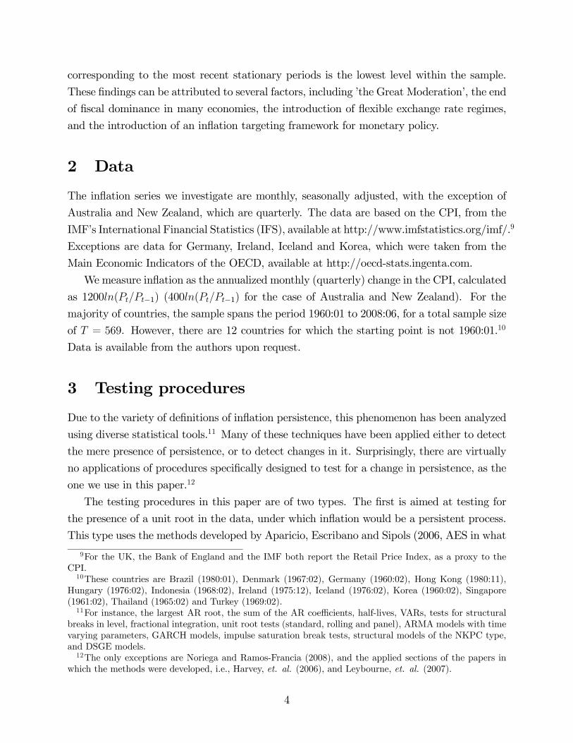
Results are presented in Table 2. We run the procedure for values of kimax = 1, 2, 3, 4
for each country, and found that for almost all countries results are robust to the value of
kimax.
Table 2 reports results for kimax = 2 for all countries but Argentina and Venezuela, for
which we set kimax to zero, and one, respectively. The selection of kimax for these two
countries was made on the basis of how well the procedure picks the apparent level breaks
present in the data, by making changes in persistence and changes in level to coincide. On this
point, LKT argue that ”In practice it is probably not unreasonable to assume that structural
breaks in the deterministic kernel dt occur at the same point(s) in the sample as changes
in persistence” (p.20), and discuss some evidence on the occurrence of this coincidence (see
Kurozumi (2005)).18
18For the case of Argentina, this value of kimax = 0 gives similar results to those of kimax = 3, 4. Wediscard results for kimax = 1, 2 since they do not correspond to the fiscal and monetary policy arrangementesmade, and contradicts previous research results (Capistrán and Ramos-Francia (2006)). A similar reasoningapplies to Venezuela.
9
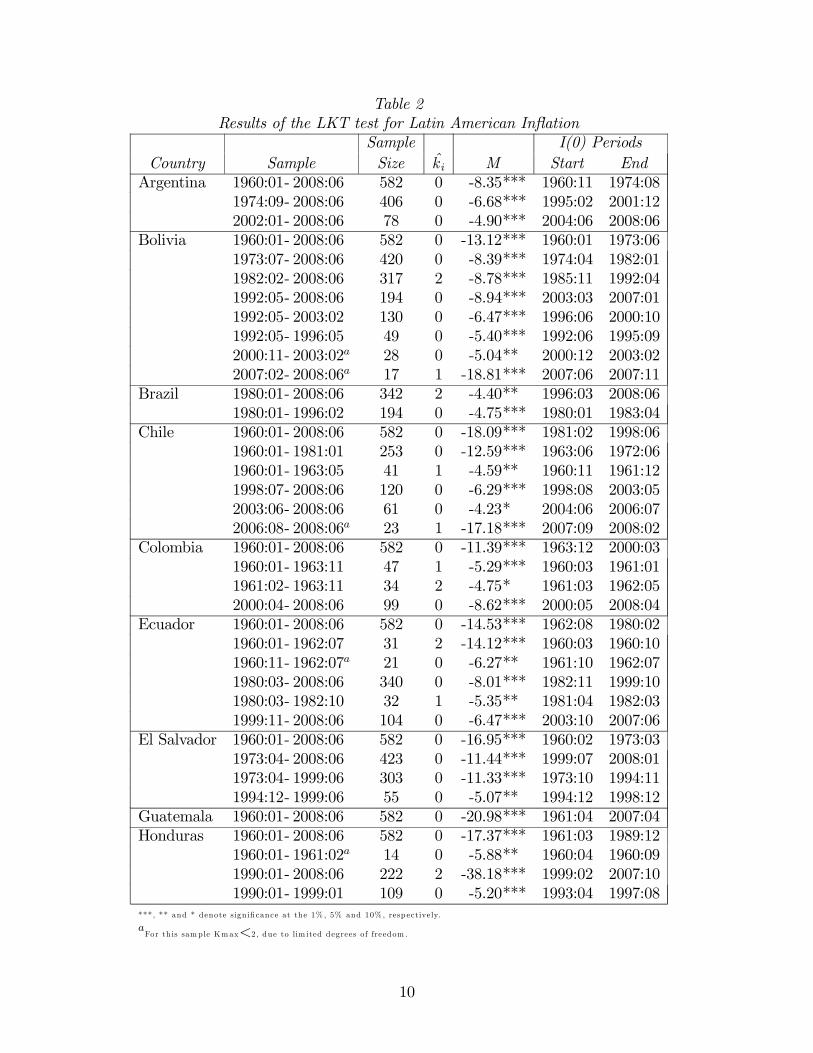
Table 2Results of the LKT test for Latin American Inflation
Sample I(0) PeriodsCountry Sample Size k i M Start EndArgentina 1960:01- 2008:06 582 0 -8.35*** 1960:11 1974:08
1974:09- 2008:06 406 0 -6.68*** 1995:02 2001:122002:01- 2008:06 78 0 -4.90*** 2004:06 2008:06
Bolivia 1960:01- 2008:06 582 0 -13.12*** 1960:01 1973:061973:07- 2008:06 420 0 -8.39*** 1974:04 1982:011982:02- 2008:06 317 2 -8.78*** 1985:11 1992:041992:05- 2008:06 194 0 -8.94*** 2003:03 2007:011992:05- 2003:02 130 0 -6.47*** 1996:06 2000:101992:05- 1996:05 49 0 -5.40*** 1992:06 1995:092000:11- 2003:02a 28 0 -5.04** 2000:12 2003:022007:02- 2008:06a 17 1 -18.81*** 2007:06 2007:11
Brazil 1980:01- 2008:06 342 2 -4.40** 1996:03 2008:061980:01- 1996:02 194 0 -4.75*** 1980:01 1983:04
Chile 1960:01- 2008:06 582 0 -18.09*** 1981:02 1998:061960:01- 1981:01 253 0 -12.59*** 1963:06 1972:061960:01- 1963:05 41 1 -4.59** 1960:11 1961:121998:07- 2008:06 120 0 -6.29*** 1998:08 2003:052003:06- 2008:06 61 0 -4.23* 2004:06 2006:072006:08- 2008:06a 23 1 -17.18*** 2007:09 2008:02
Colombia 1960:01- 2008:06 582 0 -11.39*** 1963:12 2000:031960:01- 1963:11 47 1 -5.29*** 1960:03 1961:011961:02- 1963:11 34 2 -4.75* 1961:03 1962:052000:04- 2008:06 99 0 -8.62*** 2000:05 2008:04
Ecuador 1960:01- 2008:06 582 0 -14.53*** 1962:08 1980:021960:01- 1962:07 31 2 -14.12*** 1960:03 1960:101960:11- 1962:07a 21 0 -6.27** 1961:10 1962:071980:03- 2008:06 340 0 -8.01*** 1982:11 1999:101980:03- 1982:10 32 1 -5.35** 1981:04 1982:031999:11- 2008:06 104 0 -6.47*** 2003:10 2007:06
El Salvador 1960:01- 2008:06 582 0 -16.95*** 1960:02 1973:031973:04- 2008:06 423 0 -11.44*** 1999:07 2008:011973:04- 1999:06 303 0 -11.33*** 1973:10 1994:111994:12- 1999:06 55 0 -5.07** 1994:12 1998:12
Guatemala 1960:01- 2008:06 582 0 -20.98*** 1961:04 2007:04Honduras 1960:01- 2008:06 582 0 -17.37*** 1961:03 1989:12
1960:01- 1961:02a 14 0 -5.88** 1960:04 1960:091990:01- 2008:06 222 2 -38.18*** 1999:02 2007:101990:01- 1999:01 109 0 -5.20*** 1993:04 1997:08
***, ** and * denote signifi cance at the 1% , 5% and 10% , resp ectively.
aFor th is sample Kmax<2, due to lim ited degrees of freedom .
10

Table 2Results of the LKT Test for Latin American Inflation (Cont.)
Sample I(0) PeriodsCountry Sample Size k i M Start EndMexico 1960:01- 2008:06 582 0 -12.43*** 1961:04 1972:12
1973:01- 2008:06 426 0 -5.02*** 1973:04 1981:111981:12- 2008:06 319 1 -6.33*** 2002:09 2008:04
Paraguay 1960:01- 2008:06 582 0 -15.86*** 1971:06 2003:051960:01- 1971:05 137 0 -13.84*** 1961:09 1971:031960:01- 1961:08 20 0 -7.69*** 1960:02 1960:072003:06- 2008:06 61 0 -9.17*** 2005:02 2008:062003:06- 2005:01a 20 0 -5.96** 2003:12 2004:09
Peru 1960:01- 2008:06 582 0 -10.71*** 1960:10 1977:051977:06- 2008:06 373 0 -7.25*** 1997:01 2008:051977:06- 1996:12 235 0 -7.82*** 1978:02 1982:09
Uruguay 1960:01- 2008:06 582 0 -12.91*** 1972:05 1990:011960:01- 1972:04 148 0 -6.79*** 1960:04 1972:021990:02- 2008:06 221 0 -6.23*** 2003:08 2008:041990:02- 2003:07 162 0 -5.79*** 1991:02 1994:011994:02- 2003:07 114 0 -5.65*** 1998:12 2002:011994:02- 1998:11 58 1 -4.84** 1995:07 1996:11
Venezuela 1960:01- 2008:06 582 1 -11.15*** 1962:08 1973:081960:01- 1962:07 31 1 -5.75** 1960:02 1962:071973:09- 2008:06 418 1 -9.64*** 1989:02 1996:021973:09- 1989:01 185 1 -6.88*** 1975:04 1978:121973:09- 1975:03 19 1 -15.98*** 1974:10 1975:031979:01- 1989:01 121 1 -5.88*** 1981:02 1986:121996:03- 2008:06 148 0 -6.48*** 1998:06 2007:09
***, ** and * denote sign ifi cance at the 1% , 5% and 10% , resp ectively
aFor th is sample Kmax<2, due to lim ited degrees of freedom .
In Table 2, the second column refers to the sample or subsample over which the testing
procedure is applied. bki indicates the estimated value of ki in (2), according to the BIC,while M indicates the estimated value of the test statistic in (3). The last two columns
report the beginning and end of the I(0) regions identified by the procedure. Figure 1 in the
Appendix gives a graphical representation of the results; it shows the inflation data together
with horizontal lines, which indicate an I(0) period, as identified by the LKT test. For
convenience, these lines are drawn at the mean of each of the I(0) periods they define.
In order to show the use of Table 2, let us examine some examples. The simplest case
is that of Guatemala, for which the test rejects a unit root at the 1% level from a single
application of the M test (M = −20.98, which is significant at the 1% level, using critical
11

values from LKT19), indicating that inflation is I(0) throughout (almost) the whole sample,
that is, from 1961:04 to 2007:04.20 As can be seen from Figure 1, for the case of Guatemala,
the test identifies one I(0) period, covering almost the whole sample.21 This conclusion is in
line with results from the AES unit root test.
A slightly different result obtains for El Salvador. The M test is initially applied over
the whole sample (1960:01-2008:06), detecting an interior I(0) regime between 1960:02 and
1973:03, for which the unit root null is rejected at the 1% level. This represents the ’most
prominent’ I(0) region in the data. The test is then applied over 1973:04-2008:06 and theM
statistic rejects again at the 1% level, identifying the second I(0) regime between 1999:07 and
2008:01. This represents, in turn, the ’most prominent’ I(0) region within this subsample.
The search for a further stationary regime continues by applying the test over the sam-
ple 1973:04-1999:06, which yields a third I(0) regime corresponding to the period 1973:10-
1994:11. A fourth I(0) regime is uncovered (at the 5% level) over 1994:12-1998:12 when the
test procedure is applied over the subsample 1994:12-1999:06. Hence, the procedure detects
a total of 4 I(0) regimes, which cover virtually the hole sample. We conclude that, when
allowing for the possibility of multiple changes in persistence, inflation in El Salvador can be
represented as a set of adjacent stationary periods, each fluctuating around different mean
values (see Figure 1). This is also consistent with the findings of the AES test.
As a final example consider the case of Mexico. Results from Table 2 indicate that, after
applying the procedure over the whole sample, the first I(0) regime is detected between
1961:04 and 1972:12, with a unit root being rejected at the 1% level. Searching over the
period 1973:01-2008:06 produces another rejection at the 1% level, uncovering a second I(0)
period over 1973:04-1981:11. When the procedure is applied over 1981:12-2008:06, a third
I(0) regime is detected between 2002:09 and 2008:04. Finally, no other subsamples yielded
significant tests when applied between 1981:12 and 2002:08, which implies that inflation in
Mexico switched from I(0) to I(1) in the early 1980s, switching back to I(0) in the early
2000s. Part of these results support those reported in Chiquiar et. al. (2007).
Results from Table 2 allow us to classify countries in three groups. For the first, inflation
rates are I(0) throughout, that is, with no I(1) subperiods, or, in other words, with no
changes in persistence. This is the case of Colombia, El Salvador, Guatemala and Paraguay.
In the second group there are countries for which inflation was hit by short-lived shocks,
19The critical value for T = 400 -the sample size closest to T = 582- is -4.438 at the 1% level.20Sometimes the procedure leaves out some observations, which do not contribute in attaining the double
infimum of DFG(λ, τ) according to (3). Each subsample formed by these observations is always very small,wich makes it difficult, and in many cases imposible, to apply the procedure.21Note that the procedure canot be applied over the small segments of data not covered by this I(0) period
(1960:01-1961:03 and 2007:05-2008:06), due to the limited number of available observations.
12

identified as (short) I(1) subperiods. This is the case of Bolivia (1982-1985), Ecuador (1980-
1982, 2000-2003), Honduras (1990-1993), Uruguay (1994-1998), and Venezuela (1960-1961,
1973-1975, 1979-1981). The last group consists of economies in which shocks had longer-term
effects, inducing I(1) behavior on inflation along periods of several years: Argentina (1975-
1994), Brazil (1983-1996), Chile (1972-1980), Mexico (1982-2002), and Peru (1982-1996).22
Table 7 in Section 5 summarizes these results; as can be seen, 10 out of 14 cases (71% of LA
countries in our sample) experienced persistence changes. This gives strong support to SF2.
4.2 OECD
For all countries but Australia and Iceland, a unit root is rejected by the AES J∗ test, ascan be seen from Table 3.
Table 3Results of AES Unit Root Test on OECD Countries
Country J ∗ InferenceAustralia 1.574 I(1)Austria 0.967 *** I(0)Belgium 0.850 *** I(0)Canada 0.733 *** I(0)Denmark 0.856 *** I(0)Finland 1.172 ** I(0)France 0.850 *** I(0)Germany 0.587 *** I(0)Greece 1.231 * I(0)Hungary 0.932 *** I(0)Iceland 1.434 I(1)Ireland 1.216 * I(0)Italy 0.997 *** I(0)Luxembourg 0.821 *** I(0)Netherlands 0.821 *** I(0)New Zealand 1.218 * I(0)Norway 0.733 *** I(0)Portugal 0.997 *** I(0)Spain 0.997 *** I(0)Sweden 0.760 *** I(0)Switzerland 0.762 *** I(0)Turkey 1.040 ** I(0)UK 0.850 *** I(0)USA 0.909 *** I(0)***, **,* denote rejection at the 1% , 5% and 10% level resp ective ly.
22This last group also experienced smaller shocks as those of group two: Argentina (2002-2004), Chile(1962-1963, 2006-2008), Mexico (1960-1961).
13

As with LA countries, results seem to indicate that inflation in most of the OECDeconomies has behaved in a stationary fashion, in the sense of not behaving as a unit rootprocess. Again, this result contradicts SF1.We next investigate whether there are any possible changes in persistence within the
sample for all 24 OECD countries. As with LA economies, we ran the procedure for kimax =1, ..., 4. We obtained similar results across values of kimax for all countries but Australiaand Iceland. For these two cases, the selection of kimax followed the same criterion as theone discussed for the case of LA economies. Following this criterion, the chosen value ofkimax was three for Australia and one for Iceland.Table 4 shows results from the application of the M test of LKT, and Figure 2 plots the
inflation data and the corresponding I(0) segments, as detected by the test, drawn at theirmean values, just as for the case of the LA countries above.Again, let us study our results under groups of countries. Consider the very simple case
of Austria: inflation is I(0) throughout, upon a single application of the procedure. Nextconsider the cases of Belgium, Canada, Denmark, Finland, Germany, Greece, Hungary,Norway, New Zealand, the Netherlands, Portugal, Spain, Sweden, Switzerland, Turkey, andthe UK. For these countries, inflation is I(0) throughout, but at different mean levels, whichcoincide with the set of non-overlaping I(0) segments detected by the procedure. We gatherthese countries together with Austria and form Group 1. Group 3 is formed by the rest ofthe countries (Australia, France, Ireland, Iceland, Italy, Luxembourg, and the US), all ofwhich experimented significant changes in persistence.23 For all countries in this group butAustralia, an I(1) segment is found between the early-to-mid 1970s and the 1980s. Figure2 presents a clear graphical picture of the results, while Table 7 collects results by groups ofcountries.Our results seem to support less than for the LA economies the SF2: 29% of the countries
experienced changes in persistence; for many of them, the I(1) periods occurred around theso called ’Great Inflation’ of the US. On the other hand, for the rest of OECD countries,inflation persistence was absent throughout the sample. The stationary behavior of inflationfor these countries is conformed by I(0) non-overlaping segments, the beginning and end ofwhich seem to correspond to level changes in the data.
23Note that for OECD countries, group 2 is empty, since the identified I(1) segments were rather long-lived,and therefore were allocated into Group 3 in Table 7.
14

Table 4Results of the LKT Test for OECD Inflation
Sample I(0) PeriodsCountry Sample Size k i M Start EndAustralia 1960:01- 2008:02 194 0 -5.55*** 1991:04 2007:03
1960:01- 1991:03 127 1 -6.08*** 1976:03 1983:04Austria 1960:01- 2008:06 582 0 -19.39*** 1960:02 2008:06Belgium 1960:01- 2008:06 582 0 -14.44*** 1985:05 2007:09
1960:01- 1985:04 304 0 -9.34*** 1961:08 1985:041960:01- 1961:07a 19 1 -45.36*** 1961:01 1961:05
Canada 1960:01- 2008:06 582 0 -14.30*** 1988:01 2008:031960:01- 1987:12 336 0 -8.86*** 1962:05 1972:071960:01- 1962:04 28 2 -12.02*** 1960:02 1960:081960:09- 1962:04a 20 0 -5.40** 1961:08 1962:031972:08- 1987:12 185 0 -11.49*** 1982:12 1987:111972:08- 1982:11 124 0 -9.26*** 1977:01 1982:071972:08- 1976:12 53 0 -5.37*** 1973:01 1975:11
Denmark 1967:02- 2008:06 497 0 -15.21*** 1985:05 2008:051967:02- 1985:04 219 0 -13.29*** 1967:02 1985:04
Finland 1960:01- 2008:06 582 0 -13.32*** 1992:01 2008:041960:01- 1991:12 384 0 -12.19*** 1972:11 1982:061960:01- 1972:11 154 0 -7.94*** 1961:10 1968:121969:01- 1972:11 47 0 -5.87*** 1969:04 1972:101982:07- 1991:12 114 0 -9.18*** 1983:08 1991:12
France 1960:01- 2008:06 582 0 -13.80*** 1985:08 2008:041960:01- 1985:07 307 0 -11.13*** 1962:05 1972:04
Germany 1960:02- 2008:06 581 0 -15.84*** 1993:05 2008:051960:02- 1993:04 399 2 -10.96*** 1960:05 1972:061972:07- 1993:04 250 0 -9.38*** 1972:10 1981:121983:01- 1993:04 124 0 -7.07*** 1987:01 1993:041983:01- 1986:12 48 0 -4.44** 1983:12 1985:12
Greece 1960:01- 2008:06 582 0 -12.24*** 1960:04 1979:061979:07- 2008:06 348 0 -12.20*** 1997:03 2008:061979:07- 1997:02 212 0 -7.95*** 1981:04 1991:041979:07- 1981:03a 21 0 -6.49** 1980:01 1980:071991:05- 1997:02 70 0 -6.55*** 1993:05 1996:061991:05- 1993:04a 24 0 -7.32*** 1992:02 1992:07
***, ** and * denote sign ifi cance at the 1% , 5% and 10% , resp ectively
aFor this sample Kmax<2, due to lim ited degrees of freedom .
15

Table 4Results of the LKT Test for OECD Inflation (Cont.)
Sample I(0) PeriodsCountry Sample Size k i M Start End
Hungary 1976:02- 2008:06 389 0 -10.57*** 1976:02 1988:121989:01- 2008:06 234 0 -7.79*** 1989:04 1998:051998:06- 2008:06 121 0 -7.32*** 1998:06 2008:06
Iceland 1976:02- 2008:06 389 1 -6.41*** 1990:10 2007:07Ireland 1975:12- 2008:06 391 0 -9.01*** 1990:02 2006:05Italy 1960:01- 2008:06 582 0 -11.54*** 1960:01 1972:06
1972:07- 2008:06 432 0 -11.34*** 1996:08 2006:091972:07- 1996:07 289 0 -8.79*** 1991:08 1996:062006:10- 2008:06a 21 0 -5.06* 2006:10 2008:05
Luxembourg 1960:01- 2008:06 582 0 -17.69*** 1990:12 2007:091960:01- 1990:11 371 0 -11.65*** 1960:06 1973:10
Netherlands 1960:01- 2008:06 582 2 -83.79*** 1986:12 1999:081960:01- 1986:11 323 2 -48.85*** 1980:11 1986:041960:01- 1980:10 250 0 -18.98*** 1961:10 1980:101960:01- 1961:09a 21 0 -4.77* 1960:02 1961:041999:09- 2008:06 106 0 -7.82*** 2001:06 2008:04
New Zealand 1960:01- 2008:06 194 0 -5.91*** 1991:01 2008:011960:01- 1990:04 124 1 -5.67*** 1960:04 1969:041970:01- 1990:04 84 0 -4.99*** 1970:01 1990:02
Norway 1960:01- 2008:06 582 0 -12.62*** 1964:02 1978:121960:01- 1964:01 49 2 -6.78*** 1962:05 1963:041960:01- 1962:04 28 2 -20.32*** 1960:05 1960:111979:01- 2008:06 354 0 -11.47*** 1988:07 2007:101979:01- 1988:06 114 0 -7.34*** 1983:02 1986:051979:01- 1983:01 49 0 -6.37*** 1979:10 1983:01
Portugal 1960:01- 2008:06 582 0 -14.16*** 1966:09 1992:081960:01- 1966:08 80 0 -9.89*** 1960:01 1966:081992:09- 2008:06 190 0 -11.56*** 1993:12 2008:05
Spain 1960:01- 2008:06 582 0 -10.45*** 1986:03 2008:051960:01- 1986:02 314 0 -9.64*** 1972:07 1985:041960:01- 1972:06 150 0 -8.66*** 1960:09 1972:06
Sweden 1960:01- 2008:06 582 0 -15.77*** 1964:07 1993:041960:01- 1964:06 54 0 -6.70*** 1960:02 1964:061993:05- 2008:06 182 0 -11.36*** 1993:07 2007:09
Switzerland 1960:01- 2008:06 582 0 -13.23*** 1992:12 2007:091960:01- 1992:11 395 0 -9.85*** 1976:12 1992:10
***, ** and * denote sign ifi cance at the 1% , 5% and 10% , resp ectively
aFor this sample Kmax<2, due to lim ited degrees of freedom .
16

Table 4Results of the LKT Test for OECD Inflation (Cont.)
Sample I(0) PeriodsCountry Sample Size k i M Start End
1960:01- 1976:11 203 0 -8.00*** 1961:05 1971:101960:01- 1961:04a 16 0 -4.90* 1960:06 1960:101971:11- 1976:11 61 0 -5.15*** 1971:11 1975:06
Turkey 1969:02- 2008:06 473 0 -10.89*** 1974:03 2003:031969:02- 1974:02 61 0 -6.98*** 1969:12 1973:112003:04- 2008:06 63 1 -5.19*** 2003:09 2008:03
UK 1960:01- 2008:06 582 0 -12.24*** 1991:05 2008:031960:01- 1991:04 376 0 -11.49*** 1960:07 1970:081970:09- 1991:04 248 0 -7.46*** 1977:07 1991:041970:09- 1977:06 82 0 -4.40** 1970:09 1977:06
USA 1960:01- 2008:06 582 1 -12.09*** 1981:10 2007:121960:01- 1981:09 261 2 -7.79*** 1960:08 1965:111965:12- 1981:09 190 0 -6.16*** 1967:05 1973:011965:12- 1967:04a 17 0 -5.03* 1965:12 1966:11
***, ** and * denote signifi cance at the 1% , 5% and 10% , resp ectively
aFor this sample Kmax<2, due to lim ited degrees of freedom .
4.3 Asia
For all Asian economies, the unit root is rejected by the J∗ test of AES, as shown in Table 5.
Table 5Results of AES Unit Root Test on
Asian InflationCountry J ∗ Inference
Hong Kong 0.970 ** I(0)Indonesia 0.899 *** I(0)Japan 0.850 *** I(0)Korea 1.144 ** I(0)Malaysia 0.674 *** I(0)Singapore 0.889 *** I(0)Thailand 0.991 *** I(0)***, **,* denote rejection at the 1% , 5% and 10% level resp ectively.
Since results from the M test were robust to the choice of kimax, Table 6 reports resultsfor kimax = 2.
17

Table 6Results of the LKT test for Asian Inflation
Sample I(0) PeriodsCountry Sample Size k i M Start EndHong Kong 1980:11- 2008:06 332 0 -13.59*** 1987:04 1995:09
1980:11- 1987:03 77 0 -7.88*** 1981:04 1987:031995:10- 2008:06 153 2 -11.92*** 2003:08 2007:091995:10- 2003:07 94 0 -7.72*** 1998:06 2003:051995:10- 1998:05 32 0 -6.49** 1996:01 1997:12
Indonesia 1968:02- 2008:06 485 0 -10.63*** 1970:06 2008:06Japan 1960:01- 2008:06 582 0 -17.82*** 1981:07 2008:05
1960:01- 1981:06 258 0 -11.78*** 1960:12 1981:06Korea 1960:02- 2008:06 581 0 -17.36*** 1960:05 2008:06Malaysia 1960:01- 2008:06 582 0 -16.60*** 1976:03 2008:05
1960:01- 1976:02 194 0 -12.29*** 1960:02 1972:11Singapore 1961:02- 2008:06 569 0 -15.99*** 1987:06 2007:06
1961:02- 1987:05 316 0 -15.96*** 1961:02 1972:071972:08- 1987:05 178 0 -8.70*** 1981:09 1987:051972:08- 1981:08 109 0 -6.83*** 1974:06 1981:032007:07- 2008:06a 12 0 -4.82* 2007:09 2008:06
Thailand 1965:02- 2008:06 521 0 -13.98*** 1981:05 2007:091965:02- 1981:04 195 0 -8.81*** 1965:03 1972:071972:08- 1981:04 105 0 -8.17*** 1974:06 1979:06
***, ** and * denote signifi cance at the 1% , 5% and 10% , resp ectively
aFor this sample Kmax<2, due to lim ited degrees of freedom .
As can be deducted from Table 6 (or Figure 3), Group 1 is formed by Hong Kong, Japanand Korea, for which inflation is I(0) throughout. Group 2 is formed by Indonesia, Malaysia,Singapore and Thailand. For this group the only short spell of I(1) behavior occurred duringthe early to mid 1970s. In the case of Asia, no big shocks seem to have hit inflation duringthe last decades, or, if they had, monetary policy was effective in avoiding long periods ofpersistence.
5 Discussion
First, for all countries for which a unit root is detected by the AES test, a prolonged I(1)segment is detected by the M test. However, it is clear that the AES test is not designed todetect persistence change.Table 7 summarizes the results when groups are formed according to whether inflation has
been I(0) throughout, or has switched I(0)−I(1)−I(0) with short or long I(1) segments. Ascan be seen from Table 7, Group 1 is the largest, comprising 24 countries, representing 53%of the whole sample of countries. LA countries are evenly distributed among the 3 groups.However, the majority of them has undergone either short or long changes in persistence.As for OECD countries, most of them has behaved as I(0) throughout.
18

Table 7Summary of Results
Groups General resultGroup 1LA (4): Colombia, El Salvador, Guatemala,ParaguayOECD (17): Austria, Belgium, Canada,Denmark, Finland, Germany, Greece,Hungary, Norway, New Zealand,the Netherlands, Portugal, Spain,Sweden, Switzerland, Turkey, the UKASIA (3): Hong Kong, Japan, Korea
I(0) throughout
Group 2LA (5): Bolivia, Ecuador, Honduras,Uruguay, VenezuelaASIA (4): Indonesia, Malaysia, Singapore,Thailand
I(0)− I(1)− I(0)with short I(1) segments
Group 3LA (5): Argentina, Brazil, Chile, Mexico,PeruOECD (7): Australia, France, Ireland,Iceland, Italy, Luxembourg, the US
I(0)− I(1)− I(0)with long I(1) segments
Under a different classification, for 1 country of LA (Brazil), 15 of the OECD24 and 4of Asia25, the most recent I(0) period is also the most prominent (or the first detected),according to the M test of LKT.26 This means that, for these 20 economies, the period ofthe highest price stability occurred towards the end of the sample.Finally, Tables 8-10 present the mean and standard deviation for each of the I(0)/I(1)
periods detected by the M test in chronological order for LA (Table 8), the OECD (Table9), and Asia (Table 10). Take for instance the case of Brazil. The procedure detects an I(0)segment between the beginning of the sample (1980:01) and 1983:04. For this period, themean was calculated to be 71.07 with a standard deviation of 10.53. From 1983:05 to 1996:02the LKT test detects an I(1) segment with corresponding statistics of 182.89 and 135.90.Finally, for the period 1996:03-2008:06 an I(0) period is detected with a mean of 6.52 and astandard deviation of 4.73.27 Brazil is an example of a country for which a) the most recentI(0) segment corresponds to the lowest values of the mean and the standard deviation, and2) the I(1) segment corresponds to the highest values of the mean and standard deviation.In fact, these two features hold true not only for Brazil, but also for Chile, Iceland, Peru,France, Italy, Luxembourg, and Indonesia.
24Australia, Belgium, Canada, Denmark, Finland, France, Germany, Iceland, Ireland, Luxembourg, NewZealand, Spain, Switzerland, the UK, and the US.25Japan, Malaysia, Singapore, and Thailand.26To see this, note that in Tables 2, 4 and 6, the first reported I(0) segment corresponds to the most
prominent one.27Note that this period is the one detected by the M test as the most prominent one; see Table 2.
19

It is interesting to note from Tables 8-10 that for 26 countries28, the most recent I(0)segment corresponds to the lowest value of the mean for each country. On the other hand,for 17 countries29, the I(1) segment corresponds to the highest values of the mean.30 Thesefindings seem to suggest that persistence and average inflation tend to fall -and increase- atthe same time. This implies that good policies can induce both stability and low levels ofinflation simultaneously -and viceversa.From the twelve countries with prolonged I(1) periods31, 8 of them (Argentina, Chile,
France, Ireland, Iceland, Italy, Luxembourg, and the US) experienced the beginning of highpersistence around the early to mid 1970s. On the other end of this I(1) segment, the periodknown as the ’Great Moderation’ seems to correspond only to Chile, France, and the US,for which the end of their big inflations occurred around the first half of the 1980s.32 Forthe LA countries in this group (Brazil, Mexico and Peru) the big inflations began duringthe early 1980s, and start to slow down not before the mid 1990s. For many LA and OECDcountries, the estimated dates of change in both level and persistence, seem to have a relationto changes in the operating rules of monetary policy.33
Starting from the late 1980s, the newly gained independence (or autonomy) of manycentral banks, and their adherence to monetary policy schemes that explicitly advocatedlow stable inflation like inflation targeting, set the ground for an environment of stabilityand transparent monetary policy, which quickly began to spread around the globe. By1995, eight countries (Australia, Canada, Chile, Finland, New Zealand, Spain, Sweden, andthe UK) had fixed medium term targets for inflation, and several more (Brazil, Colombia,Indonesia, Korea, Mexico, Norway, and Thailand) joined the group during the next decade.
28Australia, Brazil, Chile, Colombia, Ecuador, Peru, Belgium, Canada, Denmark, Finland, France, Ger-many, Greece, Hungary, Iceland, Italy, Luxembourg, New Zealand, Norway, Spain, Sweden, Switzerland,Turkey, the UK, Indonesia, and Japan.29Argentina, Bolivia, Brazil, Chile, Mexico, Peru, Venezuela, France, Iceland, Ireland, Italy, Luxembourg,
the US, Indonesia, Malaysia, Singapore, and Thailand.30In the case of the Asian economies with persistence changes, the I(1) segment correspond to the highest
values of the mean and the standard deviation.31Argentina, Brazil, Chile, Mexico, Peru, Australia, France, Ireland, Iceland, Italy, Luxembourg, and the
US (see Table 7).32Our results for France and the US are in line with other studies, based on different techniques, which
document drops in inflation persistence, beginning around the early 1980s. For instance, Kumar and Okimoto(2007) compute for the G7 the Modified Feasible Exact Local Whittle estimator of the order of fractionalintegration, and document a decline in persistence in the early 1980s. For the US, Beechey and Osterholm(2007), use an AR process for inflation, derived from the central bank’s optimization problem, and estimatethe path of the time-varying inflation persistence parameter over the last 50 years. Using a state-space modeland the Kalman filter, they find significant reductions in persistence, starting again in the early 80’s. Benati(2002) reaches similar conclusions using random-coefficients AR models with GARCH effects for the UKand the US. Noriega and Ramos-Francia (2008) also find significant drops in inflation persistence for the USusing both monthly and quarterly data for a larger sample. See Levin and Piger (2006) for a recent survey.33For instance, Altissimo et. al. (2006) argue that ”There is, ..., considerable evidence that breaks in the
mean of inflation occurred at times of major shifts in the monetary policy regime. The early 1990s breakscorrespond to either the adoption of inflation targeting (Benati 2006) or, ..., to the implementation of theMaastricht criterion of nominal convergence. By comparison, breaks in the early 1980s generally reflect thedisinflation policies that occurred in the United States and the United Kingdom as well as the 1979 launchof the European Monetary System (EMS), at which point the Benelux monetary union, France, Italy, andthe Netherlands, began to peg their currency to the Deutsche Mark.” (p. 587). For a discussion on the caseof LA, see Capistrán and Ramos-Francia (2006).
20

Our results seem to be consistent with the expectation of a relatively low inflation persistenceoutlook in recent years, resulting from the credibility of central banks’ commitment to attainlow inflation rates.One theoretical implication of our findings is that the evaluation of alternative mone-
tary policy frameworks, and the computation of optimal monetary policies based on modelswith built-in inflation persistence may deliver misleading indications (as indeed indicated byBenati (2002)), since inflation persistence does not seem to be a structural feature of theeconomy. However, our results can not shed light on the sources of inflation persistence,like information processing constraints faced by private agents, the structure of nominalcontracts, and the process for the structural shock hitting the economy.
21

Table 8Summary Statistics for Latin American Inflation
Std. Order ofCountry Sample Mean Dev. IntegrationArgentina 1960:11 - 1974:08 24.46 21.28 I(0)
1974:09 - 1995:01 120.51 143.57 I(1)1995:02 - 2001:12 -0.23 3.27 I(0)2002:01 - 2004:05 16.17 24.20 I(1)2004:06 - 2008:06 9.13 2.44 I(0)
Bolivia 1960:01 - 1973:06 6.78 22.97 I(0)1974:04 - 1982:01 15.73 28.99 I(0)1982:02 - 1985:10 271.08 241.73 I(1)1985:11 - 1992:04 22.80 41.64 I(0)1992:06 - 1995:09 8.32 3.13 I(0)1996:06 - 2000:10 4.88 5.23 I(0)2000:12 - 2003:02 1.59 3.34 I(0)2003:03 - 2007:01 4.86 3.31 I(0)
Brazil 1980:01 - 1983:04 71.07 10.53 I(0)1983:05 - 1996:02 182.89 135.90 I(1)1996:03 - 2008:06 6.52 4.73 I(0)
Chile 1963:06 - 1972:06 26.02 27.46 I(0)1972:07 - 1981:01 92.53 93.68 I(1)1981:02 - 1998:06 14.62 17.58 I(0)1998:08 - 2003:05 3.22 1.59 I(0)2004:06 - 2006:07 3.23 1.27 I(0)
Colombia 1963:12 - 2000:03 17.66 11.29 I(0)2000:05 - 2008:04 5.88 3.20 I(0)
Ecuador 1962:08 - 1980:02 8.57 12.91 I(0)1982:11 - 1999:10 33.30 17.97 I(0)1999:11 - 2003:09 28.33 33.34 I(1)2003:10 - 2007:06 2.61 2.53 I(0)
El Salvador 1960:02 - 1973:03 0.88 10.52 I(0)1973:10 - 1994:11 15.09 12.17 I(0)1994:12 - 1998:12 6.03 8.44 I(0)1999:07 - 2008:01 3.70 5.81 I(0)
Honduras 1961:03 - 1989:12 5.56 11.27 I(0)1990:01 - 1993:03 18.00 14.89 I(1)1993:04 - 1997:08 20.88 9.70 I(0)1999:02 - 2007:10 10.83 29.82 I(0)
Mexico 1961:04 - 1972:12 3.23 6.82 I(0)1973:04 - 1981:11 19.79 9.68 I(0)1981:12 - 2002:08 31.21 28.75 I(1)2002:09 - 2008:04 4.06 2.00 I(0)
22

Table 8Summary Statistics for Latin American Inflation (Cont.)
Std. Order ofCountry Sample Mean Dev. IntegrationParaguay 1961:09 - 1971:03 2.51 7.14 I(0)
1971:06 - 2003:05 14.65 16.76 I(0)2005:02 - 2008:06 9.33 6.46 I(0)
Peru 1960:10 - 1977:05 12.03 16.28 I(0)1978:02 - 1982:09 51.28 20.69 I(0)1982:10 - 1996:12 116.08 190.14 I(1)1997:01 - 2008:05 3.06 3.80 I(0)
Uruguay 1960:04 - 1972:02 35.71 36.94 I(0)1972:05 - 1990:01 47.91 30.93 I(0)1991:02 - 1994:01 48.16 14.45 I(0)1996:12 - 1998:11 11.79 5.13 I(1)1998:12 - 2002:01 4.28 4.13 I(0)2002:02 - 2003:07 18.91 15.69 I(1)2003:08 - 2008:04 6.97 4.33 I(0)
Venezuela 1960:02 - 1962:07 -0.48 22.70 I(0)1962:08 - 1973:08 2.04 3.47 I(0)1975:04 - 1978:12 7.11 3.53 I(0)1979:01 - 1981:01 18.45 7.06 I(1)1981:02 - 1986:12 9.79 6.41 I(0)1987:01 - 1989:01 31.73 19.14 I(1)1989:02 - 1996:02 41.69 29.84 I(0)1996:03 - 1998:05 44.75 26.41 I(1)1998:06 - 2007:09 17.53 9.46 I(0)
Table 9Summary Statistics for OECD Inflation
Std. Order ofCountry Sample Mean Dev. Integration
Australia 1960:01 - 1976:02 5.26 4.87 I(1)1976:03 - 1983:04 9.62 3.07 I(0)1984:01 - 1991:03 6.31 2.95 I(1)1991:04 - 2007:03 2.47 2.07 I(0)
Belgium 1961:08 - 1985:04 5.61 4.49 I(0)1985:05 - 2007:09 2.00 2.64 I(0)
Canada 1962:05 - 1972:07 3.21 2.26 I(0)1973:01 - 1975:11 9.89 2.77 I(0)1977:01 - 1982:07 9.71 2.83 I(0)1982:12 - 1987:11 4.15 2.23 I(0)1988:01 - 2008:03 2.38 3.24 I(0)
23

Table 9Summary Statistics for OECD Inflation (Cont.)
Std. Order ofCountry Sample Mean Dev. Integration
Denmark 1967:02 - 1985:04 8.44 8.22 I(0)1985:05 - 2008:05 2.47 2.77 I(0)
Finland 1961:10 - 1968:12 6.00 5.92 I(0)1969:04 - 1972:10 5.31 5.20 I(0)1972:11 - 1982:06 11.59 7.43 I(0)1983:08 - 1991:12 4.93 2.90 I(0)1992:01 - 2008:04 1.59 2.66 I(0)
France 1962:05 - 1972:04 4.22 3.15 I(0)1972:05 - 1985:07 9.74 3.24 I(1)1985:08 - 2008:04 2.05 1.97 I(0)
Germany 1960:05 - 1972:06 2.93 3.07 I(0)1972:10 - 1981:12 4.95 2.87 I(0)1983:12 - 1985:12 1.79 1.80 I(0)1987:01 - 1993:04 3.19 3.36 I(0)1993:05 - 2008:05 1.66 2.30 I(0)
Greece 1960:04 - 1979:06 5.78 18.18 I(0)1981:04 - 1991:04 17.12 6.65 I(0)1993:05 - 1996:06 8.99 3.03 I(0)1997:03 - 2008:06 3.44 2.58 I(0)
Hungary 1976:02 - 1988:12 7.20 9.26 I(0)1989:04 - 1998:05 21.01 13.36 I(0)1998:06 - 2008:06 6.48 4.16 I(0)
Iceland 1976:02 - 1990:09 30.88 25.65 I(1)1990:10 - 2007:07 3.67 3.04 I(0)
Ireland 1975:12 - 1990:01 9.61 9.75 I(1)1990:02 - 2006:05 2.85 2.27 I(0)2006:06 - 2008:06 4.70 0.47 I(1)
Italy 1960:01 - 1972:06 3.74 4.40 I(0)1972:07 - 1991:07 11.57 6.61 I(1)1991:08 - 1996:06 4.51 1.97 I(0)1996:08 - 2006:09 2.21 1.15 I(0)
Luxembourg 1960:06 - 1973:10 3.18 4.27 I(0)1973:11 - 1990:11 5.40 4.46 I(1)1990:12 - 2007:09 2.17 2.76 I(0)
Netherlands 1961:10 - 1980:10 5.92 7.17 I(0)1980:11 - 1986:04 7.22 31.40 I(0)1986:12 - 1999:08 0.40 20.14 I(0)2001:06 - 2008:04 1.83 1.51 I(0)
24

Table 9Summary Statistics for OECD Inflation (Cont.)
Std. Order ofCountry Sample Mean Dev. Integration
New Zealand 1960:04 - 1969:04 3.41 2.62 I(0)1970:01 - 1990:02 10.92 5.22 I(0)1991:01 - 2008:01 2.07 1.67 I(0)
Norway 1964:02 - 1978:12 6.67 6.17 I(0)1979:10 - 1983:01 11.46 4.34 I(0)1983:02 - 1986:05 5.76 1.70 I(0)1988:07 - 2007:10 2.24 3.51 I(0)
Portugal 1960:01 - 1966:08 2.67 7.06 I(0)1966:09 - 1992:08 14.17 13.69 I(0)1993:12 - 2008:05 2.99 2.56 I(0)
Spain 1960:09 - 1972:06 6.31 7.16 I(0)1972:07 - 1985:04 14.33 7.18 I(0)1986:03 - 2008:05 4.02 2.59 I(0)
Sweden 1960:02 - 1964:06 3.01 3.40 I(0)1964:07 - 1993:04 7.09 6.45 I(0)1993:07 - 2007:09 1.28 2.46 I(0)
Switzerland 1961:05 - 1971:10 3.81 2.55 I(0)1971:11 - 1975:06 7.96 5.69 I(0)1976:12 - 1992:10 3.35 3.48 I(0)1992:12 - 2007:09 0.96 2.15 I(0)
Turkey 1969:12 - 1973:11 13.10 14.12 I(0)1974:03 - 2003:03 43.50 27.58 I(0)2003:09 - 2008:03 9.21 4.54 I(0)
UK 1960:07 - 1970:08 4.00 4.12 I(0)1970:09 - 1977:06 13.27 7.76 I(0)1977:07 - 1991:04 7.61 6.06 I(0)1991:05 - 2008:03 2.80 2.13 I(0)
USA 1960:08 - 1965:11 1.32 1.61 I(0)1967:05 - 1973:01 4.44 1.72 I(0)1973:02 - 1981:09 8.99 3.70 I(1)1981:10 - 2007:12 3.12 2.67 I(0)
25

Table 10Summary Statistics for Asian Inflation
Std. Order ofCountry Sample Mean Dev. IntegrationHong Kong 1981:04 - 1987:03 6.97 7.23 I(0)
1987:04 - 1995:09 9.00 4.27 I(0)1998:06 - 2003:05 -3.15 5.77 I(0)2003:08 - 2007:09 1.45 4.95 I(0)
Indonesia 1968:02 - 1970:05 18.29 63.88 I(1)1970:06 - 2008:06 11.47 15.07 I(0)
Japan 1960:12 - 1981:06 7.10 8.01 I(0)1981:07 - 2008:05 0.85 3.36 I(0)
Korea 1960:05 - 2008:06 8.70 13.75 I(0)Malaysia 1960:02 - 1972:11 1.16 6.60 I(0)
1972:12 - 1976:02 9.31 10.94 I(1)1976:03 - 2008:05 3.22 4.30 I(0)
Singapore 1961:02 - 1972:07 1.24 7.98 I(0)1972:08 - 1974:05 20.74 21.32 I(1)1974:06 - 1981:03 3.71 6.78 I(0)1981:09 - 1987:05 0.79 4.84 I(0)1987:06 - 2007:06 1.49 3.14 I(0)
Thailand 1965:03 - 1972:07 2.35 5.33 I(0)1972:08 - 1974:05 20.28 11.56 I(1)1974:06 - 1979:06 6.03 7.61 I(0)1981:05 - 2007:09 3.56 4.84 I(0)
6 Conclusions
Using time series techniques, we have analyzed the dynamics of persistence in inflation ratesfor 45 countries, using (mostly) monthly seasonally adjusted data from 1960 to 2008. Ourresults indicate that for half of the countries analyzed, inflation is stationary throughoutthe sample. For this group of countries, the level around which (nonpersistent) inflation hasfluctuated does not seem to be constant. For many countries in this group, particularly thosebelonging to the OECD, the lowest levels of inflation correspond to the most recent periods,i.e. from the 1980s to the end of the sample for some countries, or from the 1990s to the endof the sample for others. This phenomenon could be related to the ’Great Moderation’, andthe introduction of inflation targeting as a framework for monetary policy.On the other hand, the presence of persistence change seems to be pervasive: for half
of countries mixtures of low and high persistence episodes were detected along the sampleperiod, most prominently among Latin American economies. For the great majority ofcountries in this second group, the high persistence periods are also those with the highestinflation mean and standard deviation within the sample.
26

7 Appendix
Figure 1Results of the LKT Tests for Latin American InflationArgentina Bolivia
-100
-50
0
50
100
150
Jan-
60
Jan-
64
Jan-
68
Jan-
72
Jan-
76
Jan-
80
Jan-
84
Jan-
88
Jan-
92
Jan-
96
Jan-
00
Jan-
04
Jan-
08
-50
-10
30
70
110
150
Jan-
60
Jan-
64
Jan-
68
Jan-
72
Jan-
76
Jan-
80
Jan-
84
Jan-
88
Jan-
92
Jan-
96
Jan-
00
Jan-
04
Jan-
08
Brazil Chile
-50
-10
30
70
110
Jan-
60
Jan-
64
Jan-
68
Jan-
72
Jan-
76
Jan-
80
Jan-
84
Jan-
88
Jan-
92
Jan-
96
Jan-
00
Jan-
04
Jan-
08
-50
-20
10
40
70
Jan-
60
Jan-
64
Jan-
68
Jan-
72
Jan-
76
Jan-
80
Jan-
84
Jan-
88
Jan-
92
Jan-
96
Jan-
00
Jan-
04
Jan-
08
Colombia Ecuador
-30
0
30
60
90
Jan-
60
Jan-
64
Jan-
68
Jan-
72
Jan-
76
Jan-
80
Jan-
84
Jan-
88
Jan-
92
Jan-
96
Jan-
00
Jan-
04
Jan-
08
-50
-10
30
70
110
150
Jan-
60
Jan-
64
Jan-
68
Jan-
72
Jan-
76
Jan-
80
Jan-
84
Jan-
88
Jan-
92
Jan-
96
Jan-
00
Jan-
04
Jan-
08
El Salvador Guatemala
-40
-20
0
20
40
60
Jan-
60
Jan-
64
Jan-
68
Jan-
72
Jan-
76
Jan-
80
Jan-
84
Jan-
88
Jan-
92
Jan-
96
Jan-
00
Jan-
04
Jan-
08
-80
-40
0
40
80
120
Jan-
60
Jan-
64
Jan-
68
Jan-
72
Jan-
76
Jan-
80
Jan-
84
Jan-
88
Jan-
92
Jan-
96
Jan-
00
Jan-
04
Jan-
08
27

Figure 1Results of the LKT Tests for Latin American Inflation (Cont.)
Honduras Mexico
-30
-10
10
30
50
70Ja
n-60
Jan-
64
Jan-
68
Jan-
72
Jan-
76
Jan-
80
Jan-
84
Jan-
88
Jan-
92
Jan-
96
Jan-
00
Jan-
04
Jan-
08
-20
20
60
100
140
Jan-
60
Jan-
64
Jan-
68
Jan-
72
Jan-
76
Jan-
80
Jan-
84
Jan-
88
Jan-
92
Jan-
96
Jan-
00
Jan-
04
Jan-
08
Paraguay Peru
-20
0
20
40
60
80
100
Jan-
60
Jan-
64
Jan-
68
Jan-
72
Jan-
76
Jan-
80
Jan-
84
Jan-
88
Jan-
92
Jan-
96
Jan-
00
Jan-
04
Jan-
08
-50
30
110
190
270
350
Jan-
60
Jan-
64
Jan-
68
Jan-
72
Jan-
76
Jan-
80
Jan-
84
Jan-
88
Jan-
92
Jan-
96
Jan-
00
Jan-
04
Jan-
08
Uruguay Venezuela
-50
0
50
100
150
200
Jan-
60
Jan-
64
Jan-
68
Jan-
72
Jan-
76
Jan-
80
Jan-
84
Jan-
88
Jan-
92
Jan-
96
Jan-
00
Jan-
04
Jan-
08
-50
-20
10
40
70
100
Jan-
60
Jan-
64
Jan-
68
Jan-
72
Jan-
76
Jan-
80
Jan-
84
Jan-
88
Jan-
92
Jan-
96
Jan-
00
Jan-
04
Jan-
08
28

Figure 2Results of the LKT Tests for OECD InflationAustralia Austria
-3
2
7
12
17
22
1960
Q1
1964
Q1
1968
Q1
1972
Q1
1976
Q1
1980
Q1
1984
Q1
1988
Q1
1992
Q1
1996
Q1
2000
Q1
2004
Q1
2008
Q1
-5
0
5
10
15
20
Jan-
60
Jan-
64
Jan-
68
Jan-
72
Jan-
76
Jan-
80
Jan-
84
Jan-
88
Jan-
92
Jan-
96
Jan-
00
Jan-
04
Jan-
08
Belgium Canada
-5
0
5
10
15
20
Jan-
60
Jan-
64
Jan-
68
Jan-
72
Jan-
76
Jan-
80
Jan-
84
Jan-
88
Jan-
92
Jan-
96
Jan-
00
Jan-
04
Jan-
08
-5
0
5
10
15
20
Jan-
60
Jan-
64
Jan-
68
Jan-
72
Jan-
76
Jan-
80
Jan-
84
Jan-
88
Jan-
92
Jan-
96
Jan-
00
Jan-
04
Jan-
08
Denmark Finland
-10
0
10
20
30
Jan-
60
Jan-
64
Jan-
68
Jan-
72
Jan-
76
Jan-
80
Jan-
84
Jan-
88
Jan-
92
Jan-
96
Jan-
00
Jan-
04
Jan-
08
-10
0
10
20
30
Jan-
60
Jan-
64
Jan-
68
Jan-
72
Jan-
76
Jan-
80
Jan-
84
Jan-
88
Jan-
92
Jan-
96
Jan-
00
Jan-
04
Jan-
08
France Germany
-5
0
5
10
15
20
Jan-
60
Jan-
64
Jan-
68
Jan-
72
Jan-
76
Jan-
80
Jan-
84
Jan-
88
Jan-
92
Jan-
96
Jan-
00
Jan-
04
Jan-
08
-5
-1
3
7
11
15
Jan-
60
Jan-
64
Jan-
68
Jan-
72
Jan-
76
Jan-
80
Jan-
84
Jan-
88
Jan-
92
Jan-
96
Jan-
00
Jan-
04
Jan-
08
29

Figure 2Results of the LKT Tests for OECD Inflation (Cont.)
Greece Hungary
-20
-10
0
10
20
30
40
50Ja
n-60
Jan-
64
Jan-
68
Jan-
72
Jan-
76
Jan-
80
Jan-
84
Jan-
88
Jan-
92
Jan-
96
Jan-
00
Jan-
04
Jan-
08
-10
10
30
50
70
Jan-
60
Jan-
64
Jan-
68
Jan-
72
Jan-
76
Jan-
80
Jan-
84
Jan-
88
Jan-
92
Jan-
96
Jan-
00
Jan-
04
Jan-
08
Iceland Ireland
-10
20
50
80
110
Feb-
60
Feb-
64
Feb-
68
Feb-
72
Feb-
76
Feb-
80
Feb-
84
Feb-
88
Feb-
92
Feb-
96
Feb-
00
Feb-
04
Feb-
08
-10
0
10
20
30
40
Jan-
60
Jan-
64
Jan-
68
Jan-
72
Jan-
76
Jan-
80
Jan-
84
Jan-
88
Jan-
92
Jan-
96
Jan-
00
Jan-
04
Jan-
08
Italy Luxembourg
-10
0
10
20
30
Jan-
60
Jan-
64
Jan-
68
Jan-
72
Jan-
76
Jan-
80
Jan-
84
Jan-
88
Jan-
92
Jan-
96
Jan-
00
Jan-
04
Jan-
08
-10
0
10
20
Jan-
60
Jan-
64
Jan-
68
Jan-
72
Jan-
76
Jan-
80
Jan-
84
Jan-
88
Jan-
92
Jan-
96
Jan-
00
Jan-
04
Jan-
08
Netherlands New Zealand
-20
-5
10
25
40
Jan-
60
Jan-
64
Jan-
68
Jan-
72
Jan-
76
Jan-
80
Jan-
84
Jan-
88
Jan-
92
Jan-
96
Jan-
00
Jan-
04
Jan-
08
-3
4
11
18
25
32
1960
Q1
1964
Q1
1968
Q1
1972
Q1
1976
Q1
1980
Q1
1984
Q1
1988
Q1
1992
Q1
1996
Q1
2000
Q1
2004
Q1
2008
Q1
30
Figure 2Results of the LKT Tests for OECD Inflation (Cont.)
Norway Portugal
-10
0
10
20
30Ja
n-60
Jan-
64
Jan-
68
Jan-
72
Jan-
76
Jan-
80
Jan-
84
Jan-
88
Jan-
92
Jan-
96
Jan-
00
Jan-
04
Jan-
08
-20
0
20
40
60
80
Jan-
60
Jan-
64
Jan-
68
Jan-
72
Jan-
76
Jan-
80
Jan-
84
Jan-
88
Jan-
92
Jan-
96
Jan-
00
Jan-
04
Jan-
08
Spain Sweden
-15
-5
5
15
25
35
Jan-
60
Jan-
64
Jan-
68
Jan-
72
Jan-
76
Jan-
80
Jan-
84
Jan-
88
Jan-
92
Jan-
96
Jan-
00
Jan-
04
Jan-
08
-10
0
10
20
30
Jan-
60
Jan-
64
Jan-
68
Jan-
72
Jan-
76
Jan-
80
Jan-
84
Jan-
88
Jan-
92
Jan-
96
Jan-
00
Jan-
04
Jan-
08
Switzerland Turkey
-5
0
5
10
15
20
Jan-
60
Jan-
64
Jan-
68
Jan-
72
Jan-
76
Jan-
80
Jan-
84
Jan-
88
Jan-
92
Jan-
96
Jan-
00
Jan-
04
Jan-
08
-20
10
40
70
100
130
160
Jan-
60
Jan-
64
Jan-
68
Jan-
72
Jan-
76
Jan-
80
Jan-
84
Jan-
88
Jan-
92
Jan-
96
Jan-
00
Jan-
04
Jan-
08
U.K USA
-8
2
12
22
32
Jan-
60
Jan-
64
Jan-
68
Jan-
72
Jan-
76
Jan-
80
Jan-
84
Jan-
88
Jan-
92
Jan-
96
Jan-
00
Jan-
04
Jan-
08
-8
-3
2
7
12
17
22
Jan-
60
Jan-
64
Jan-
68
Jan-
72
Jan-
76
Jan-
80
Jan-
84
Jan-
88
Jan-
92
Jan-
96
Jan-
00
Jan-
04
Jan-
08
31

Figure 3Results of the LKT Tests for Asian Inflation
Hong Kong Indonesia
-20
-12
-4
4
12
20
28Ja
n-60
Jan-
64
Jan-
68
Jan-
72
Jan-
76
Jan-
80
Jan-
84
Jan-
88
Jan-
92
Jan-
96
Jan-
00
Jan-
04
Jan-
08
-50
-25
0
25
50
75
100
Jan-
60
Jan-
64
Jan-
68
Jan-
72
Jan-
76
Jan-
80
Jan-
84
Jan-
88
Jan-
92
Jan-
96
Jan-
00
Jan-
04
Jan-
08
Japan Korea
-10
0
10
20
30
40
Jan-
60
Jan-
64
Jan-
68
Jan-
72
Jan-
76
Jan-
80
Jan-
84
Jan-
88
Jan-
92
Jan-
96
Jan-
00
Jan-
04
Jan-
08
-30
-10
10
30
50
70
90
Jan-
60
Jan-
64
Jan-
68
Jan-
72
Jan-
76
Jan-
80
Jan-
84
Jan-
88
Jan-
92
Jan-
96
Jan-
00
Jan-
04
Jan-
08
Malaysia Singapore
-20
-10
0
10
20
30
40
Jan-
60
Jan-
64
Jan-
68
Jan-
72
Jan-
76
Jan-
80
Jan-
84
Jan-
88
Jan-
92
Jan-
96
Jan-
00
Jan-
04
Jan-
08
-20
-10
0
10
20
30
40
50
Jan-
60
Jan-
64
Jan-
68
Jan-
72
Jan-
76
Jan-
80
Jan-
84
Jan-
88
Jan-
92
Jan-
96
Jan-
00
Jan-
04
Jan-
08
Thailand
-10
0
10
20
30
40
50
Jan-
60
Jan-
64
Jan-
68
Jan-
72
Jan-
76
Jan-
80
Jan-
84
Jan-
88
Jan-
92
Jan-
96
Jan-
00
Jan-
04
Jan-
08
32

8 References
Altissimo, F., L. Bilke, A. Levin, T. Mathä and B. Mojon (2006), Sectorial and AggregateInflation Dynamics in the Euro Area” Journal of the European Economic Association, 4(2—3),585—593.Aparicio, F., A. Escribano and A. E. Sipols (2006), “Range Unit-Root (RUR) Tests:
Robust Against Nonlinearities, Error Distributions, Structural Breaks and Outliers” Journalof Time Series Analysis, 27(4), 545-576.Ball, L. (2006) "Has Globalization Changed Inflation’", NBER Working Paper 12687.Batini N. (2002) “Euro Area Inflation Persistence” Working Paper 201, European Central
Bank.Batini N. and E. Nelson (2002), “The Lag from Monetary Policy Actions to Inflation:
Friedman Revisited”, Discussion Paper 6, Bank of England.Beechey, M. and P. Osterholm (2007), “The Rise and Fall of U.S. Inflation Persistence”,
Working Paper 2007:18, Department of Economics Uppsala University.Benati, L. (2002), “Investigating Inflation Persistence Across Monetary Regimes I: Em-
pirical Evidence”, Working Paper, Bank of England.Benati, L. (2006), “UK Monetary Regimes and Macroeconomic Stylized Facts”, Working
Paper No. 290, Bank of England.Borio, C., W. English and A. Filardo (2003), “A Tale of Two Perspectives: Old or New
Challenges for Monetary Policy?”, Bank for International Settlements Papers No. 19.Burridge, P. and D. Hristova (2008), “Consistent Estimation and Order Selection for
Nonstationary Autoregressive Processes with Stable Innovations”, Journal of Time SeriesAnalysis, 29(4), 695-718.Caggiano, G. and E. Castelnuovo (2007), “Investigating Inflation Persistence in the ACF
Domain”, unpublished, University of Padua.Capistrán, C. and M. Ramos-Francia (2006), “Inflation Dynamics in Latin America”,
Working Paper 2006-11, Banco de Mexico, forthcoming in Contemporary Economic Policy.Chiquiar, D., A. E. Noriega, and M. Ramos-Francia (2007), “A Time Series Approach to
Test a Change in Inflation Persistence: The Mexican Experience”, Banco de México WorkingPapers 2007-01. Forthcoming in Applied Economics.Coenen, G. (2007), “Inflation Persistence and Robust Monetary Policy Design”, Journal
of Economic Dynamics and Control, 31, 111-140.Cogley, T. and T.J. Sargent (2001), “Evolving Post-World War II Inflation Dynamics”,
NBER Macroeconomics Annual, 16.Culver, S. and D. Papell (1997), “Is There a Unit Root in The Inflation Rate? Evidence
From Sequential Break and Panel Data Models”, Journal of Applied Econometrics, 12, 435-444.Gadea, M. and L. Mayoral (2006), “The Persistence of Inflation in OECD Countries:
A Fractionally Integrated Approach”, International Journal of Central Banking, March (4),51-104.Hall, R., (1999), "Comment on Rethinking the role of NAIRU in monetary policy: Im-
plications of model formulation and uncertainty", by A. Estrella and F. Mishkin, in J. B.Taylor ed., Monetary Policy Rules, University of Chicago Press.
33

Harvey, D.I., S.J. Leybourne and A.M.R. Taylor (2006), “Modified Tests for a Change inPersistence”, Journal of Econometrics, 134, 441-469.Kim, J. (2000), “Detection of Change in Persistence of a Linear Time Series”, Journal of
Econometrics, 95, 97-116.Kontonikas, A. (2004), “Inflation and Inflation Uncertainty in the United Kingdom, Ev-
idence from GARCH Modelling”, Economic Modelling, 21, 525-543.Kumar, M. and T. Okimoto (2007), “Dynamics of Persistence in International Inflation
Rates”, Journal of Money, Credit and Banking, 39(6), 1457-1479.Kurozumi, E. (2005), “Detection of Structural Change in the Long-Run Persistence in a
Univariate Time Series”, Oxford Bulletin of Economics and Statistics, 67(2), 181-206.Levin, A. and J.M. Piger (2006), "Is Inflation Persistence Intrinsic in Industrial Economies?",
mimeo.Leybourne, S., T. Kim and A. M. Taylor (2007), “Detecting Multiple Changes in Persis-
tence”, Studies in Nonlinear Dynamics and Econometrics”, 11(3), 1-32.Leybourne, S., R. Taylor and T. Kim (2006), “CUSUM of Squares-based Tests for a
Change in Persistence”, Journal of Time Series Analysis, 28(3), 408-433.Ng, S. and P. Perron (2001), “Lag Length Selection and the Construction of Unit Root
Tests with Good Size and Power”, Econometrica, 69(6), 1519-54.Noriega, A. and M. Ramos-Francia (2008), “A Note on the Dynamics of Persistence in
US Inflation”, Banco de México Working Paper 2008-12.O’Reilly, G. and K. Whelan (2004), “Has Euro-Area Inflation Persistence Changed Over
Time?” Working Paper 335, European Central Bank.Perron, P. and Z. Qu (2007), “A Simple Modification to Improve the Finite Sample
Properties of Ng and Perron’s Unit Root Tests”, Economics Letters, 94, 12-19.Pivetta, F. and R. Reis (2007), “The Persistence of Inflation in the United States”,
Journal of Economic Dynamics and Control, 31(4), 1326-1358.Primiceri, G. E. (2006), "Why inflation rose and fell: Policy-makers’ beliefs and U. S.
postwar stabilization policy", Quarterly Journal of Economics, 121 (3), 867-901.Rogoff, K. (2003) "Globalization and Global Disinflation", Federal Reserve Bank of
Kansas City Economic Review, 4th Quarter, 88(4), 45-78.Santos, C. andM. A. Oliveira (2007), “Assessing French inflation persistence with impulse
saturation break tests and automatic general-to-specific modelling”, Working Paper 10/2007,Facultad de Economia e Gestão, Universidade Católica Portuguesa, Porto.Sargent, T., N. Williams and T. Zha, (2004), "Shocks and government beliefs: the rise
and fall of American inflation", NBER working paper 10764.Trehan, B. and C. Walsh, (1988), "Common Trends, the Government Budget Constraint
and Revenue Smoothing", Journal of Economic Dynamics and Control, 12, 425-444.________, (1990), Seigniorage and Tax Smoothing in the United States 1914-1986,
Journal of Monetary Economics, 25 (1), 97-112.
34


![[ES] Manejadores de persistencia](https://img.pdfslide.es/doc/110x75/557b81d0d8b42a2d298b5379/es-manejadores-de-persistencia.jpg)