Embed Size (px)
Citation preview

TERMODINAMICA DE AGUJEROS NEGROS CON COMPORTAMIENTO
ASINTOTICO NO ESTANDAR
MOISES FELIPE BRAVO GAETE 1
Una tesis presentada en cumplimiento parcial de
los requisitos para el grado de
Doctor en Matematicas
Instituto de Matematica y Fısica
Universidad de Talca
MAYO 2015
1 Sostenido en parte por Beca Doctorado Nacional 2012-CONICYT N 21120271.

Indice general
1. Introduccion 1
2. Preliminares 6
2.1. Geometrıa Diferencial . . . . . . . . . . . . . . . . . . . . . . . . . . . . . . . . . . . . . . . . 6
2.1.1. Espacio tangente . . . . . . . . . . . . . . . . . . . . . . . . . . . . . . . . . . . . . . . 7
2.1.2. Espacio dual . . . . . . . . . . . . . . . . . . . . . . . . . . . . . . . . . . . . . . . . . 8
2.1.3. Tensores y operaciones con tensores . . . . . . . . . . . . . . . . . . . . . . . . . . . . 8
2.1.4. Metrica . . . . . . . . . . . . . . . . . . . . . . . . . . . . . . . . . . . . . . . . . . . . 9
2.1.5. Derivada covariante . . . . . . . . . . . . . . . . . . . . . . . . . . . . . . . . . . . . . 10
2.1.6. Geodesicas . . . . . . . . . . . . . . . . . . . . . . . . . . . . . . . . . . . . . . . . . . 11
2.1.7. Curvatura, tensores de Riemann y Ricci . . . . . . . . . . . . . . . . . . . . . . . . . . 12
2.1.8. Formas diferenciales . . . . . . . . . . . . . . . . . . . . . . . . . . . . . . . . . . . . . 14
2.1.9. Derivada de Lie y vectores de Killing . . . . . . . . . . . . . . . . . . . . . . . . . . . . 16
2.2. Relatividad General . . . . . . . . . . . . . . . . . . . . . . . . . . . . . . . . . . . . . . . . . 17
2.2.1. Principio de Equivalencia . . . . . . . . . . . . . . . . . . . . . . . . . . . . . . . . . . 18
2.2.2. Tensor de energıa-momento Tµν y las ecuaciones de Einstein . . . . . . . . . . . . . . 19
2.2.3. Formulacion Lagrangiana . . . . . . . . . . . . . . . . . . . . . . . . . . . . . . . . . . 20
2.3. Agujeros negros clasicos . . . . . . . . . . . . . . . . . . . . . . . . . . . . . . . . . . . . . . . 21
2.3.1. Agujero negro de Schwarzschild . . . . . . . . . . . . . . . . . . . . . . . . . . . . . . . 21
2.3.2. Agujero negro de Reissner-Nordstrom . . . . . . . . . . . . . . . . . . . . . . . . . . . 32
2.3.3. Agujero negro de Kerr . . . . . . . . . . . . . . . . . . . . . . . . . . . . . . . . . . . . 36
3. Agujeros negros en presencia de un campo escalar no mınimamente acoplado a la cur-
vatura escalar 44
3.1. Agujeros negros en presencia de un campo escalar no mınimamente acoplado a la curvatura
escalar conforme . . . . . . . . . . . . . . . . . . . . . . . . . . . . . . . . . . . . . . . . . . . 46
3.1.1. Agujeros negros en presencia de (D − 1)-formas . . . . . . . . . . . . . . . . . . . . . . 50
3.2. Gravedad de Lovelock . . . . . . . . . . . . . . . . . . . . . . . . . . . . . . . . . . . . . . . . 52
3.3. Agujeros negros asintoticamente AdS con horizonte planar en presencia de un campo escalar
no mınimamente acoplado a la curvatura escalar . . . . . . . . . . . . . . . . . . . . . . . . . 54
4. Primera ley de la termodinamica para agujeros negros asintoticamente Lifshitz 82
4.1. Termodinamica de los agujeros negros . . . . . . . . . . . . . . . . . . . . . . . . . . . . . . . 83
4.1.1. Leyes de la termodinamica de los agujeros negros . . . . . . . . . . . . . . . . . . . . . 84
4.1.2. Entropıa de Wald . . . . . . . . . . . . . . . . . . . . . . . . . . . . . . . . . . . . . . . 85
4.1.3. Formalismos para obtener la masa de soluciones de agujeros negros . . . . . . . . . . . 87
4.2. Teorıas gravitatorias masivas . . . . . . . . . . . . . . . . . . . . . . . . . . . . . . . . . . . . 94
4.2.1. Accion de Fierz-Pauli . . . . . . . . . . . . . . . . . . . . . . . . . . . . . . . . . . . . 95
4.2.2. Gravedad masiva topologica . . . . . . . . . . . . . . . . . . . . . . . . . . . . . . . . . 96
4.2.3. Nueva gravedad masiva . . . . . . . . . . . . . . . . . . . . . . . . . . . . . . . . . . . 98
4.3. Calculo de la masa de agujeros negros considerando el formalismo cuasilocal . . . . . . . . . . 100
4.4. Primera ley y formula de Cardy generalizada para agujeros negros de Lifshitz en tres dimensiones105
4.5. Agujeros negros asintoticamente Lifshitz en presencia de un campo electrico . . . . . . . . . . 115
5. Teorıa de Horndeski 126
5.1. Agujeros negros en presencia de una fuente particular de la teorıa de Horndeski . . . . . . . . 127
5.2. Agujeros negros de Lifshitz con un campo escalar dependiente del tiempo en una teorıa de
Horndeski . . . . . . . . . . . . . . . . . . . . . . . . . . . . . . . . . . . . . . . . . . . . . . . 132
5.3. Termodinamica de un agujero negro BTZ con una fuente de Horndeski . . . . . . . . . . . . . 137
6. Conclusiones y comentarios 146
7. Apendice 149
palabra
AGRADECIMIENTOS
Sinceramente, es difıcil escribir estas lıneas pues son variadas las personas e instituciones que, de alguna
u otra forma, han sido importantes a lo largo de estos casi cuatro anos de trabajo. En primer lugar, quisiera
agradecer al Instituto de Matematica y Fısica por darme la oportunidad de continuar mis estudios. Asimismo,
a la Universidad de Talca y la Comision Nacional de Investigacion Cientıfica y Tecnologica (CONICYT) por
su financiamiento. A modo personal, quisiera dar infinitas gracias a mi tutor, Doctor Mokhtar Hassaıne, por
ensenarme que el trabajo duro generan, tarde o temprano, resultados fructıferos.
Tambien quisiera dar mi agradecimiento a los profesores: Doctor Ricardo Baeza, Doctor Luis Huerta,
Doctor Mikhail S. Plyushchay y Doctor Jorge Zanelli, por ser una parte esencial dentro de mi proceso
doctoral.
Agradezco tambien a mis amigos y companeros de postgrado, tanto de Magıster como de Doctorado,
ası como tambien de todos los profesores y personas que forman parte del Instituto y de la Universidad, por
sus valiosos consejos y ensenanzas.
Por ultimo, y no menos importante, quisiera dar mi incondicional gratitud a mi familia y seres queridos,
en especial a mis padres, Marıa y Moises, por cultivarme la constancia y, a modo personal, obsequiarme lo
mas valioso que se puede entregar a un hijo: el amor y deseo de aprender. A mi querida hermana, Marıa
Alicia, por sus incontables y valiosas conversaciones. A Catherine, por su amor, paciencia, y ser un pilar
fundamental en mi vida. Finalmente, a mi tıo, Patricio Manuel, que dejo este mundo hace diez anos, su
apoyo y conviccion fueron las bases para seguir este camino.
palabra

A mi familia y seres queridos.

palabra
Capıtulo 1
Introduccion
El objetivo de esta tesis es la busqueda y el analisis de soluciones de agujeros negros, considerando teorıas
que modifican las ecuaciones de Einstein presentes en los artıculos [1–6]. Estas ecuaciones forman parte de
la teorıa de la Relatividad General [7–9], descubierta en 1915 por Albert Einstein, luego de un laborioso
trabajo. Su esencia se encuentra en que sus ecuaciones, ademas de su belleza y simplicidad, permiten estudiar
la interaccion entre la materia y la gravedad, asociando esta ultima a un concepto puramente geometrico. Es
mas, esta teorıa ha incorporado una unidad denominada espacio-tiempo, la cual ha pasado de ser un escenario
estatico donde ocurre la fısica a ser una parte mas de la fısica [10]. En estricto rigor, en las ecuaciones aparece
un tensor Gµν (que determina la geometrıa) conocido como tensor de Einstein, construido mediante el escalar
de Ricci (o curvatura escalar), y el tensor de Ricci; ambos se pueden definir como una medida de la curvatura
del espacio-tiempo. La componente asociada en describir la fuente de materia, que induce esta curvatura, se
encuentra definida por el tensor de energıa-momento Tµν . Cada uno de estos tensores se obtienen por medio
de una accion funcional S, donde se presenta una seccion correspondiente al campo gravitacional, conocida
como accion de Einstein-Hilbert, y una contribucion proveniente de los campos de materia [79].
Modificaciones a las ecuaciones de Einstein contemplan, por ejemplo, la inclusion de una constante
cosmologica Λ [11,12], ası como la introduccion de terminos de curvaturas superiores a la gravedad [54,98,121].
En este contexto, estudiaremos cada una de estas ideas encontrando interesantes familias de soluciones de
agujeros negros. Estos los podemos definir intuitivamente como una region finita del espacio-tiempo capaz
de generar un campo gravitatorio tal que ninguna partıcula (ni siquiera la luz) puede escapar, envuelta por
una region denominada horizonte de eventos.
Por otra parte, el estudio de teorıas gravitatorias nos entrega informacion sobre teorıas cuanticas de
campos fuertemente acopladas (TCC). En particular, las TCC’s relevantes en muchas aplicaciones presentes
en fısica corresponden a aquellas invariantes bajo el grupo conforme, esto es: escalamiento, transformaciones
de Lorentz y traslaciones de la teorıa de la Relatividad Especial. A estas clases de TCC’s se les denominan
teorıas de campos conformes (CFT por sus siglas en ingles). Esta invariancia conforme nos permite traducirla
a una simetrıa geometrica de un espacio-tiempo denominado anti-de Sitter (AdS) [21–24], el cual junto
con el espacio-tiempo de Sitter (dS) y Minkowski, corresponden a los tres espacio-tiempos maximalmente
1
simetricos [12]. Esta dualidad se conoce en la literatura como correspondencia AdS/CFT. Asimismo, la
presencia de agujeros negros en las ecuaciones de Einstein son trascendentales en esta correspondencia.
Gracias a los trabajos elaborados por J. Bardeen, B. Carter y S. Hawking [78] en la decada de 1970, nos
permiten dar luces al hecho que los agujeros negros se comportan como un sistema termodinamico, y que
existen cuatro leyes que gobiernan su comportamiento, las cuales poseen una similitud con las cuatro leyes
de la termodinamica clasica. Mas aun, S. Hawking mostro que los agujeros negros son capaces de emitir
radiacion, con una temperatura caracterıstica [76]; y J. Bekenstein se percato que poseen una entropıa, la
cual es proporcional al area del horizonte de eventos [77]. Cada una de estas propiedades esta ligada a la
geometrıa de los agujeros negros, permitiendo obtener la termodinamica de teorıas cuanticas de campos
fuertemente acopladas, las cuales son en general difıciles de trabajar [24]. De lo anterior, resulta necesaria la
busqueda y el estudio de mecanismos que nos permitan calcular los parametros termodinamicos asociados a
los agujeros negros.
Desde hace algunos anos se ha tratado de extender la correspondencia AdS/CFT estudiando teorıas de
campos fuertemente acopladas con escalamiento anisotropico, tales como en fısica de materia condensada [70],
donde la gravedad dual de estos sistemas corresponde a los denominados espacio-tiempos de Lifshitz [71],
admitiendo una simetrıa de escala distinta entre las coordenadas espaciales y temporales por medio de un
parametro conocido como exponente dinamico z, donde el caso z = 1 corresponde a AdS. La extension
natural de la construccion de [71] corresponde a buscar configuraciones que sean asintoticamente el espacio-
tiempo de Lifshitz, siendo conocidos con el nombre de agujeros negros de Lifshitz, encontrandose una variedad
importante de estas soluciones en la literatura, ver por ejemplo [72–75].
En la correspondencia AdS/CFT estandar, se ha mostrado que la metrica AdS resuelve las ecuaciones
de Einstein con una constante cosmologica negativa sin la necesidad de una fuente de materia [25, 35]. Sin
embargo, de manera de sostener la metrica de Lifshitz con z 6= 1, estas ecuaciones no son suficientes. Lo
anterior conlleva la introduccion de fuentes extra de materia, tales como un campo de Proca [72], modelos
electrodinamicos mas generales [73], o considerar correcciones de curvaturas cuadraticas a la gravedad de
Einstein [74,75].
Por otra parte, desde el punto de vista de la termodinamica de agujeros negros, en la decada de 1990,
R. Wald [80, 81] construyo una forma diferencial que se identifica a una carga de Noether, la cual esta ınti-
mamente vinculada a la entropıa de un agujero negro. De la misma manera, se estudiaron formalismos para
obtener la masa de estas soluciones. Uno de los primeros acercamientos fue escribir la accion de Einstein-
Hilbert en terminos de una formulacion Hamiltoniana, conocida en la literatura como formalismo ADM
(R. Arnowitt, S. Deser y C. Misner) [83], donde la accion gravitacional se encuentra complementada con
un termino de superficie [79, 84], el cual es esencial para calcular la masa de soluciones asintoticamente
planas, tales como el agujero negro de Schwarzschild; sin embargo, para espacio-tiempos mas generales se
ha mostrado que es insuficiente. Otro procedimiento corresponde al formalismo ADT (L. Abbott, S. Deser
y B. Tekin) [86–88], por medio de la construccion de un potencial denominado ADT y de la linealizacion de
las ecuaciones de movimiento, permitiendo calcular la masa de soluciones tales como la de Schwarzschild-
AdS [25, 35], cuyo comportamiento asintotico es de curvatura constante negativa. Recientemente, se ha
2
formulado un nuevo metodo que considera una generalizacion cuasilocal del formalismo ADT [92, 93] cuyo
resultado principal corresponde al hecho que el potencial ADT fuera de la cascara (en el sentido que la
metrica base obtenida de la linealizacion no necesariamente debe satisfacer las ecuaciones de movimiento en
el vacıo) se puede expresar en funcion de un termino de superficie, y un potencial denominado de Noether
fuera de la cascara. A modo de ejemplo, este formalismo ha sido eficiente con el fin de obtener la masa de
soluciones de agujeros negros de Lifshitz considerando correcciones de curvaturas cuadraticas a la gravedad
de Einstein [74, 75], donde por medio de la temperatura de Hawking [76] y entropıa de Wald [80, 81], se
verifica que se sostiene la primera ley de la termodinamica de agujeros negros.
En la practica, considerar teorıas con una fuente de materia es un problema no trivial, debido fundamen-
talmente a la conjetura de no-pelo [36, 40], la cual establece que todas las soluciones de agujeros negros en
las ecuaciones de Einstein-Maxwell de gravitacion y electromagnetismo, pueden ser caracterizadas solamente
por la masa, carga y momento angular. Una manera de evitar tal conjetura es agregando un campo escalar
no mınimamente acoplado a la gravedad, descubierto en la decada de 1970 por N. Bocharova, K. Bron-
nikov y V. Melnikov [41], y J. Bekenstein [42]. Al estudiar campos escalares no mınimamente acoplados,
nos referimos a un campo escalar Φ con termino cinetico − 12∇µΦ∇µΦ, junto con un termino acoplado al
escalar de Ricci de la forma ξRΦ2, donde ξ es el parametro de acoplamiento no minimal. Esta teorıa es
capaz de sostener configuraciones de agujeros negros, cuyo primer resultado conocido es la solucion BBMB
(Bocharova-Bronnikov-Melnikov-Bekenstein). No obstante, esta solucion posee como deficiencia el hecho que
el campo escalar diverge en el horizonte. Una manera de eludir este inconveniente es mediante la inclusion
de una constante cosmologica a las ecuaciones de movimiento, cuyo efecto es impulsar esta singularidad
detras del horizonte de eventos [47]. Ademas, es posible extender la topologıa del horizonte de eventos, cuyas
soluciones son conocidas como agujeros negros topologicos, encontrandose configuraciones con una topologıa
esferica o hiperbolica dependiendo del signo de la constante cosmologica [48, 50]. Hay que tener presente
que para todos estos casos, la dimension del espacio-tiempo es cuatro y el parametro de acoplamiento no
minimal ξ es siempre conforme (ξ = 1/6); esto significa que la seccion de materia, asociada al campo escalar,
posee una invariancia conforme. A su vez, esto conlleva a que la curvatura escalar R puede ser constante, o
incluso nula, dependiendo de la teorıa, simplificando sustancialmente las ecuaciones de campo. Asimismo, la
introduccion de dos 3-formas no trivialmente acopladas al campo escalar [51,52] permite extender esta cons-
truccion para un parametro de acoplamiento no minimal ξ y dimension del espacio-tiempo D arbitrarios [53].
Desde el punto de vista de la correspondencia AdS/CFT, lo anterior es providencial para la construccion de
agujeros negros con un horizonte planar, debido a que estas soluciones han recibido un gran interes en la
busqueda de un mejor entendimiento en superconductores no convencionales [67–69]. Bajo este contexto, en
orden de reproducir el diagrama de fase de estos superconductores, el sistema debe admitir agujeros negros
con un pelo escalar a baja temperatura, el cual debe desaparecer a una alta temperatura.
El modelo asociado a un campo escalar no mınimamente acoplado, expuesto en el parrafo anterior, forma
parte de una teorıa conocida como la accion de Horndeski [119], correspondiente a la accion tensor-escalar
mas general cuyas ecuaciones de movimiento respecto a la metrica y al campo escalar son a lo mas ecuaciones
diferenciales de segundo orden en dimension cuatro. En particular, estudiamos otra subclase de esta teorıa
3
donde la fuente de materia se encuentra conformada por un campo escalar Φ junto con su termino cinetico
usual, ademas de un acoplamiento cinetico no minimal de la forma Gµν∇µΦ∇νΦ. Una de las primeras
soluciones de agujeros negros sin constante cosmologica fue encontrada en [125], donde el cuadrado de la
derivada del campo escalar es negativo fuera del horizonte de eventos. Tal como en el caso no mınimamente
acoplado, este problema ha sido evitado mediante la inclusion de una constante cosmologica, obteniendo
en [127] soluciones asintoticamente localmente AdS (o incluso planar). La version electricamente cargada de
estos agujeros negros fue estudiada en [128]. A su vez, esta teorıa admite soluciones estaticas no triviales con
simetrıa esferica considerando un campo escalar dependiente del tiempo [129]. Mas aun, para una eleccion
adecuada de las constantes de acoplamiento, se obtiene una configuracion stealth, esto es, una solucion no
trivial donde tanto la seccion gravitatoria como de materia son identicamente nulas, sobre la metrica de
Schwarzschild. En todos estos ejemplos, a fin de eludir el teorema de no-pelo presente en [124], se estudian
soluciones donde la componente radial de la corriente conservada se anula, simplificando considerablemente
las ecuaciones de campo.
El esquema de esta tesis es como sigue y explica de manera mas profunda cada una de las ideas expues-
tas anteriormente. En el capıtulo 2 exponemos, en primer lugar, ciertas nociones correspondientes a una
importante rama de la matematica conocida como Geometrıa Diferencial. Posteriormente, estudiamos la Re-
latividad General [7–9] y las ecuaciones de Einstein. Finalizando el capıtulo, damos a conocer agujeros negros
clasicos presentes en la literatura en dimension cuatro, comenzando con la solucion de Schwarzschild [15]
(correspondiente a la unica solucion estatica con simetrıa esferica en el vacıo), luego examinaremos soluciones
cargadas electricamente (conocidas usualmente como de Reissner-Nordstrom [17,18]), y el agujero negro de
Kerr [19,20] descubierto en la decada de los sesenta, el cual incluye un momento angular.
En el capıtulo 3 analizamos de manera concreta la teorıa asociada a un campo escalar no mınimamente
acoplado a la curvatura escalar, su evolucion a lo largo del tiempo y su implicancia en la busqueda de agujeros
negros. Asimismo, estudiamos como la inclusion de (D − 2)-campos, correspondientes a (D − 1)-formas,
permiten extender la constante de acoplamiento no minimal ξ, encontrando configuraciones planares para las
ecuaciones de Einstein [53]. Luego, exponemos un caso particular de la teorıa gravitatoria de Lovelock [55,56].
Para ser mas precisos, los coeficientes que aparecen en la gravedad de Lovelock se fijan para que la teorıa
posea un unico vacıo de AdS, fijando la constante cosmologica, generando un conjunto de teorıas gravitatorias
indexadas por un entero k [61], donde k = 1 corresponde al Lagrangiano de Einstein-Hilbert con una
constante cosmologica. Al final del capıtulo, damos a conocer nuestros resultados descubiertos en [1, 2].
El capıtulo 4 hace referencia a la termodinamica asociada a los agujeros negros. Una parte importante de
este trabajo se concentra en la primera ley de la termodinamica y en formalismos que nos permitan obtener
tanto la masa como la entropıa de estas soluciones. Adicionalmente, mostramos teorıas gravitatorias alter-
nativas mediante la inclusion de terminos de curvatura superior a las ecuaciones de Einstein. En particular,
estamos interesados en una teorıa tridimensional denominada nueva gravedad masiva [108], la cual ha sido
estudiada intensamente durante los ultimos anos y ha permitido la obtencion de dos interesantes clases de
soluciones de agujeros negros, caracterizadas por un exponente dinamico z = 1 [114], la cual corresponde a
una solucion asintoticamente AdS, y una solucion con z = 3 [74]. Asimismo, presentamos algunos ejemplos
4

concretos del calculo de la masa de agujeros negros conocidos en la literatura por medio del formalismo
cuasilocal. Posteriormente, damos a conocer nuestras soluciones presentes en [3, 4].
El capıtulo 5 revela la subclase de la teorıa de Horndeski [119] dada por la accion de Einstein-Hilbert junto
a una constante cosmologica, ademas de un campo escalar conformado por su termino cinetico usual y un
acoplamiento cinetico no minimal. Adicionalmente, mostramos soluciones de agujeros negros recientemente
descubiertos, entregando las bases para dar a conocer nuestros resultados presentes en [5, 6].
Finalmente, en el capıtulo 6 consideramos las conclusiones y comentarios finales. Se ha agregado tambien
un apendice para explicar de mejor forma algunas formulas de la seccion 4.5.
Artıculos aceptados y publicados presentes en la tesis:
1. M. Bravo Gaete and M. Hassaıne, Topological black holes for Einstein-Gauss-Bonnet gravity with a
nonminimal scalar field, Phys. Rev. D 88, 104011 (2013) [arXiv:1308.3076 [hep-th]].
2. M. Bravo Gaete and M. Hassaıne, Planar AdS black holes in Lovelock gravity with a nonminimal scalar
field, JHEP 1311, 177 (2013) [arXiv:1309.3338 [hep-th]].
3. E. Ayon-Beato, M. Bravo Gaete, F. Correa, M. Hassaıne, M. M. Juarez-Aubry and J. Oliva, First
law and anisotropic Cardy formula for three-dimensional Lifshitz black holes, Phys. Rev. D 91, 064006
(2015) [arXiv:1501.01244 [gr-qc]].
4. M. Bravo Gaete and M. Hassaıne, Thermodynamics of charged Lifshitz black holes with quadratic
corrections, Phys. Rev. D 91, 064038 (2015)[arXiv:1501.03348 [hep-th]].
5. M. Bravo Gaete and M. Hassaıne, Lifshitz black holes with a time-dependent scalar field in Horndeski
theory, Phys. Rev. D 89, 104028 (2014) [arXiv:1312.7736 [hep-th]].
6. M. Bravo Gaete and M. Hassaıne, Thermodynamics of a BTZ black hole solution with an Horndeski
source, Phys. Rev. D 90, 024008 (2014) [arXiv:1405.4935 [hep-th]].
5
Capıtulo 2
Preliminares
En todos los sentidos, tanto la matematica como la fısica son dos disciplinas hermanas que se necesitan
una de la otra, pues para analizar cualquier fenomeno resulta necesario un conjunto de reglas que traten de
explicarlo, ası como tambien de expresiones matematicas que las sostengan. En particular, la teorıa de la
Relatividad General no se encuentra ajena a esta alianza. Es por ello que este capıtulo se centra en estos
temas y esta organizado como sigue. En la seccion 2.1 estudiamos los conceptos asociados a la Geometrıa
Diferencial, cimentando las bases para las ecuaciones de Einstein, para luego en la seccion 2.2 dar a conocer
el Principio de Equivalencia, junto con la formulacion Lagrangiana de la gravedad de Einstein. Finalmente,
en la seccion 2.3 se exponen soluciones de agujeros negros clasicos presentes en la literatura.
2.1. Geometrıa Diferencial
Antes de tener en consideracion los conceptos fısicos relacionados a la Relatividad General y las ecuaciones
de Einstein, se debe tener en cuenta ciertas nociones de caracter matematico, tales como por ejemplo el
concepto de variedad diferenciable, el cual, intuitivamente, es un conjunto que localmente puede ser descrito
como Rn. Formalmente tenemos [12,13]
Definicion 1 Una variedad topologica de dimension n es un espacio topologico de Haussdorff M, tal que
para todo punto p ∈M existe un entorno U homeomorfo a un abierto de Rn. Algunos ejemplos de variedades
son
1. El mismo Rn, incluyendo la recta R y el plano R2.
2. La n-esfera Sn, la cual puede ser vista como el lugar geometrico de todos los puntos de una cierta
distancia fija desde el origen en Rn+1.
3. El N-Toro Tn, el cual resulta tomando un cubo n-dimensional e identificando sus lados opuestos.
Definicion 2 Una carta, denotada por (U , φ), de la variedad topologica M es un par compuesto por un
abierto U de M y un homeomorfismo φ : U −→ φ(U) ⊂ Rn.
6

Definicion 3 Un atlas C∞ de la variedad M es un conjunto de cartas (Uα, φα) tal que
1. Cubre completamente a la variedad M, esto es M =⋃α Uα.
2. Satisfacen la compatibilidad de cartas, esto es, si Uα ∩ Uβ 6= ∅, entonces la funcion de transicion entre
ambas φα φ−1β : φβ(Uα ∩ Uβ) −→ φα(Uα ∩ Uβ) corresponde a una funcion C∞ entre abiertos en Rn.
Definicion 4 Una variedad diferenciable C∞ es una variedad topologica M que posee un atlas C∞.
Definicion 5 Llamaremos a las coordenadas xµ del punto p de la variedadM, asociada a una carta (Uα, φα)
que la contenga, a las coordenadas de φ(p) ∈ Rn.
Definicion 6 Consideremos una funcion f :M−→ R, denotaremos de la misma forma a su correspondiente
en coordenadas locales, esto es f(xu) := f φ−1(xµ) = f(p). Una funcion f es C∞ si y solo si f φ−1 lo es.
Una vez elaborado este trabajo preparatorio, a continuacion estudiaremos varios tipos de estructuras aso-
ciadas a la variedad M.
2.1.1. Espacio tangente
Consideremos una parametrizacion γ(t) de clase C∞ de una curva en la variedadM, esto es una aplicacion
γ : I ⊂ R −→M,
con γ(t0) = p ∈M. Sea D el conjunto de funciones diferenciables sobre M en p.
Definicion 7 El vector tangente a la curva γ en t0 es una aplicacion v(f)∣∣γ(t0)
: D −→ R dada por
v(f)∣∣γ(t0)
=d(f γ)
dt
∣∣∣t0, f ∈ D.
Definicion 8 Un vector tangente en p es el vector tangente en t = t0 para alguna curva γ sobre M, con
γ(t0) = p.
Definicion 9 El conjunto de todos los vectores tangentes a la variedad M de dimension n en el punto p es
un espacio vectorial cuya dimension coincide con la de la variedad, denominado espacio vectorial tangente
al punto p, el cual lo denotaremos como TpM. Dada su condicion de espacio vectorial, un punto p = γ(t0)
se puede escribir como
p =
n∑
µ=1
vµeµ∣∣p
:= vµeµ∣∣p,
donde utilizaremos el convenio de sumacion de Einstein y el conjunto de vectores eµ∣∣p
corresponden a una
base coordenada del espacio TpM, dada por
eµ∣∣p
=d(f φ−1)
dxµ
∣∣∣p.
De ahora en adelante, salvo que existan confusiones, omitiremos el termino eµ∣∣p
y lo escribiremos simplemente
como eµ.
7
2.1.2. Espacio dual
Una vez que hemos establecido el concepto de espacio vectorial tangente, podemos definir otro espacio
vectorial asociado de igual dimension.
Definicion 10 El espacio vectorial dual, el cual denotaremos como T ∗pM, es el espacio de todas las aplica-
ciones lineales ω del espacio tangente TpM a R, esto es
ω : TpM−→ R. (2.1.1)
Definicion 11 Dada una base eµ del espacio tangente TpM, podemos construir un conjunto de vectores
duales θν de T ∗pM tal que
θν(eµ) = δνµ =
1 si µ = ν,
0 si µ 6= ν.
Este conjunto es linealmente independiente y, por lo tanto, forman una base, conocida como base dual. Por
consiguiente, todo vector dual ω de T ∗pM puede ser escrito como ω = ωµθµ.
En la literatura, es comun que los elementos de TpM tambien sean conocidos como vectores covariantes y
los elementos del espacio vectorial dual T ∗pM como vectores contravariantes.
2.1.3. Tensores y operaciones con tensores
Una generalizacion de los vectores y vectores duales corresponde a la nocion de tensor.
Definicion 12 Un tensor T de tipo (k, l) es una aplicacion multilineal sobre una coleccion de vectores duales
y vectores a R
T : T ∗pM× ...× T ∗pM︸ ︷︷ ︸k veces
×TpM× TpM× ...× TpM︸ ︷︷ ︸l veces
−→ R,
donde × denota el producto Cartesiano, mientras que la multilinealidad corresponde al hecho que el tensor
actua linealmente sobre cada uno de sus argumentos.
Con la definicion anterior, tenemos que un tensor tipo (0, 0) corresponde a un escalar, un (1, 0)-tensor es un
vector y un (0, 1)-tensor es un vector dual.
El espacio de todos los (k, l)-tensores es un espacio vectorial, sumando tensores y multiplicando un tensor
por un escalar real. Dado lo anterior, es necesaria la definicion de una base, para ello utilizaremos la operacion
conocida como producto tensorial, denotada como ⊗.
Definicion 13 Sea T un (k, l)-tensor y S un (m,n)-tensor, definimos un (k+m, l+ n)-tensor T ⊗ S como
T ⊗ S(ω(1), . . . , ω(k+m), v(1), . . . , v(l+n)) := T (ω(1), . . . , ω(k), v(1), . . . , v(l))
× S(ω(k+1), . . . , ω(k+m), v(l+1), . . . , v(l+n)), (2.1.2)
donde los ω(i) y v(j) son distintos vectores y vectores duales, con
i = 1, . . . , k +m, j = 1, . . . , l + n.
8
Ahora, es posible construir la base para el (k, l)-tensor considerando el siguiente conjunto
eµ1⊗ . . .⊗ eµk ⊗ θν1 ⊗ . . .⊗ θνl. (2.1.3)
Notemos que si la dimension de la variedad es n, entonces la base tendra nk+l elementos. Los tensores del
tipo (k, 0) corresponden a tensores contravariantes, mientras que los tensores (0, l) son tensores covariantes.
Finalmente, podemos escribir un (k, l)-tensor arbitrario como
T = Tµ1µ2...µkν1ν2...νl eµ1
⊗ . . .⊗ eµk ⊗ θν1 ⊗ . . .⊗ θνl . (2.1.4)
De ahora en adelante denotaremos el tensor T por sus componentes Tµ1µ2...µkν1ν2...νl . Asimismo, podemos
realizar operaciones a estos tensores de tal manera que mantengan el caracter tensorial:
1. Dados dos (k, l)-tensores T y S podemos considerar la suma y la multiplicacion por un escalar, esto es
debido a su condicion de espacio vectorial.
2. Dado un tensor T de componentes Tµ1µ2...µkν1ν2...νl en una base arbitraria, se define su parte simetrica
en los ındices covariantes al tensor de componentes
Tµ1µ2...µk(ν1ν2...νl) :=
1
l!
∑
σ
Tµ1µ2...µkσ(ν1)σ(ν2)...σ(νl), (2.1.5)
donde la suma se extiende a todas las permutaciones σ de los ındices ν1, ν2, . . . , νl. Analogamente, su
parte antisimetrica en los ındices covariantes es
Tµ1µ2...µk[ν1ν2...νl] :=
1
l!
∑
σ
(−1)σ Tµ1µ2...µkσ(ν1)σ(ν2)...σ(νl), (2.1.6)
y (−1)σ toma valores positivos o negativos dependiendo si la permutacion es par o impar.
3. Dado un tensor T de componentes Tµ1µ2...µkν1ν2...νl , podemos realizar la operacion contraccion con
respecto al ındice i-esimo como el tensor de componentes Tµ1µ2...αi...µkν1ν2...αi...νl . Notemos que si
tenemos un (k, l) -tensor, la operacion contraccion lo convierte en un (k − 1, l − 1)- tensor.
2.1.4. Metrica
Dados los conceptos y definiciones anteriores, veremos a continuacion un tensor muy especial conocido
como tensor metrico, el cual representa el campo gravitacional en las ecuaciones de Einstein.
Definicion 14 Un tensor metrico, denotado por gµν , en un (0, 2)-tensor simetrico no degenerado, esto es,
el determinante de la metrica |g| := |gµν | es no nulo.
Esto nos permite definir la metrica inversa gµν de la siguiente forma
gµνgµσ = gτσgτµ = δµσ , (2.1.7)
la cual es simetrica, debido a la definicion de gµν . Esta nueva herramienta nos permite realizar la operacion
de subir y bajar ındices, convirtiendo tensores contravariantes en covariantes y viceversa. Ademas, es posible
9

representar el tensor metrico de la forma ds2 = gµνdxµdxν , el cual se conoce en la literatura como elemento
de lınea.
Llamaremos la signatura de un tensor metrico a la diferencia entre los valores propios positivos y negativos
que posea. Cuando el signo de la metrica para una variedad de dimension n es de la forma (+,+, . . . ,+) la
metrica se conoce como Riemanniana, mientras que si el signo es (−,+, . . . ,+) decimos que es Lorentziana.
Notemos que para la primera metrica su signatura es n, mientras que la segunda es n− 2.
Dada una variedad M y un vector vµ ∈ TpM, una metrica Lorentziana permite separar este espacio en
tres tipos de vectores, estos son:
1. Temporales, tales que vµvµ = gµνvµvν < 0.
2. Espaciales, tales que vµvµ = gµνvµvν > 0.
3. Nulos, tales que vµvµ = gµνvµvν = 0.
Lo anterior define un cono de luz en un punto p de la variedad, esquematizado en la Figura 2.1.
Figura 2.1: Cono de Luz.
2.1.5. Derivada covariante
Una conexion afın ∇, conocida como derivada covariante, es una asignacion que permite relacionar a
cada (k, l)- tensor en otro tensor de tipo (k, l + 1), la cual debe tener las siguientes propiedades:
1. Linealidad: ∇(aT + bS) = a∇T + b∇S.
2. Regla de Leibniz: ∇(T ⊗ S) = (∇T )⊗ S + T ⊗ (∇S).
10
3. Conmuta con la contraccion, esto es ∇µ(Tλλρ
)= (∇T )
λλρ .
4. Sobre una funcion φ, tenemos que ∇µφ = ∂µφ.
Donde a, b ∈ R y T, S son tensores. Formalmente, para un tensor T cuyas componentes son Tµ1µ2...µkν1ν2...νl ,
la derivada covariante es
∇σTµ1µ2...µkν1ν2...νl = ∂σT
µ1µ2...µkν1ν2...νl + Γµ1
σλTλµ2...µk
ν1ν2...νl + Γµ2
σλTµ1λ...µk
ν1ν2...νl
+ . . .+ ΓµkσλTµ1µ2...λ
ν1ν2...νl − Γλσν1Tµ1µ2...µk
λν2...νl − Γλσν2Tµ1µ2...µk
ν1λ...νl
− · · · − ΓλσνlTµ1µ2...µk
ν1ν2...λ, (2.1.8)
y la conexion Γλµν se conoce como los Sımbolos de Christoffel, los cuales estan en funcion de la metrica gµν
y sus primeras derivadas, esto es
Γλµν =1
2gλσ (∂µgνσ + ∂νgσµ − ∂σgµν) . (2.1.9)
2.1.6. Geodesicas
En el espacio Rn, las rectas son curvas preferidas por dos razones. La primera de ellas es que estas curvas
corresponden a la distancia mas corta entre dos puntos. La segunda es el hecho que las rectas son las unicas
donde el vector tangente es transportado paralelamente a lo largo de la misma curva [10]. Cada uno de estos
conceptos se pueden generalizar considerando una variedad M y la metrica gµν .
Si nos enfocamos en primer lugar en la distancia mas corta entre dos puntos, debemos tener presente la
siguiente definicion:
Definicion 15 Una geodesica metrica es la curva xµ(t) entre dos puntos p y q cuya longitud s, expresada
como
s =
∫ q
p
dt
√gµν
dxµ
dt
dxν
dt, (2.1.10)
es estacionaria bajo pequenas variaciones tanto de la curva como de la metrica. Esta geodesica corresponde
a la curva por la cual δs = 0, representada por las ecuaciones de Euler-Lagrange
∂t
[δL
δ (∂txµ)
]− δL
δxµ= 0, (2.1.11)
con L = dsdt =
√gµν
dxµ
dtdxν
dt y ∂t = ddt .
Ahora, consideremos la siguiente accion
S =1
2
∫ q
p
dt gµν xµx ν , (2.1.12)
donde, por motivos de simplicidad, se define x µ := dxµ
dt . Notemos que la accion (2.1.12) es justamente la
ecuacion de distancia (2.1.10) sin la raız cuadrada. Utilizando las ecuaciones de Euler-Lagrange (2.1.11)
obtenemos
∂t
(δS
δx µ
)=
1
2
(∂β gµλx
λx β + ∂α gτν xτ x α + gµλx
λ + gτν xτ), (2.1.13)
δS
δxµ=
1
2∂τgµν x
µx ν . (2.1.14)
11
Reordenando y re-indexando los terminos, tenemos que
gτσxσ +
1
2(∂σgτρ + ∂ρgστ − ∂τgρσ) x σ x ρ = 0. (2.1.15)
Si multiplicamos por la componente metrica gµτ y recordamos la definicion de los sımbolos de Christoffel
(2.1.9) obtenemos
xµ + Γµσρxσxρ = 0. (2.1.16)
Por otro lado, para la generalizacion del concepto del transporte paralelo, consideremos lo siguiente:
Definicion 16 Una geodesica afın es aquella curva xµ(t) donde su vector tangente uµ = xµ(t) es transpor-
tado paralelamente a lo largo de la curva, esto es
uν∇νuµ = xµ + Γµσρxσxρ = 0. (2.1.17)
Notemos que las ecuaciones (2.1.17) y (2.1.16) son equivalentes, dado que hemos considerando una cone-
xion de la forma (2.1.9). En otras palabras, se tiene que las geodesicas metricas y afines coinciden.
2.1.7. Curvatura, tensores de Riemann y Ricci
De manera natural, tenemos una idea vaga del concepto de lo que es curvatura, nos es intuitivo si lo
consideramos en el plano cartesiano, pero en un espacio de dimensiones mayores y en una variedad el concepto
ya es difıcil. En primer lugar, consideremos la siguiente definicion:
Definicion 17 Una variedad M se dice curva si el transporte paralelo de un vector a traves de una curva
cerrada resulta un vector diferente al retornar al punto de salida.
Dado que tenemos la definicion del transporte paralelo dada por la ecuacion (2.1.17), la curvatura debe
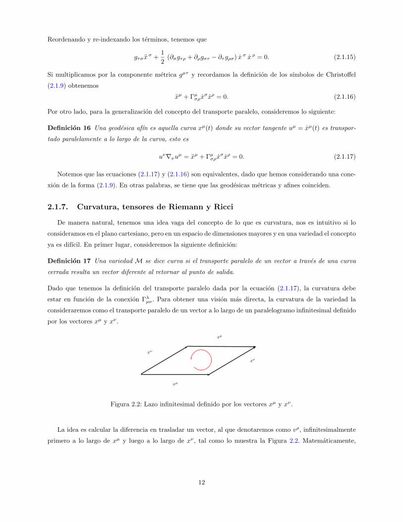
estar en funcion de la conexion Γλµν . Para obtener una vision mas directa, la curvatura de la variedad la
consideraremos como el transporte paralelo de un vector a lo largo de un paralelogramo infinitesimal definido
por los vectores xµ y xν .
xµ
xµ
xν
xν
Figura 2.2: Lazo infinitesimal definido por los vectores xµ y xν .
La idea es calcular la diferencia en trasladar un vector, al que denotaremos como vρ, infinitesimalmente
primero a lo largo de xµ y luego a lo largo de xν , tal como lo muestra la Figura 2.2. Matematicamente,
12

corresponde a calcular el conmutador [∇µ,∇ν ] de derivadas covariantes actuando sobre vρ, es decir:
[∇µ,∇ν ]vρ = ∇µ∇ν vρ −∇ν ,∇µ vρ,
= ∂µ(∇νvρ)− Γλµν∇λvρ + Γρµσ∇νvρ − (µ↔ ν),
= ∂µ∂νvρ + (∂µΓρνσ)vσ + Γρνσ∂µv
ρ − Γλµν∂λvρ − ΓλµνΓρλσv
σ + Γρµσ∂νvσ + ΓρµσΓσνλv
λ − (µ↔ ν),
= Rρ σµνvσ − 2Γλ[µν]∇λvρ,
= Rρ σµνvσ − Tλµν∇λvρ, (2.1.18)
donde Rρ σµν corresponde al tensor de Riemann, el cual mide la diferencia del transporte paralelo a lo largo
de un paralelogramo infinitesimal, y es una medida de la curvatura encerrada en el paralelogramo. Mientras
que Tλµν es el tensor de Torsion, que es la parte antisimetrica y mide hasta que punto el paralelogramo se
encuentra cerrado. Dado lo anterior, el tensor de Riemann es dado por
Rρσµν = ∂µΓρνσ − ∂νΓρµσ + ΓσµλΓλνσ − ΓρνλΓλµσ. (2.1.19)
Asimismo, dada una metrica gµν , podemos realizar la operacion tensorial de bajar ındices de la forma
Rρσµν = gρλRλσµν , (2.1.20)
obteniendose las siguientes propiedades:
1. De las ecuaciones (2.1.19) y (2.1.20), tenemos que Rρσµν es un tensor antisimetrico al intercambiar los
dos primeros ındices, ası como tambien los dos ultimos:
Rρσµν = −Rσρµν , (2.1.21)
Rρσµν = −Rρσνµ. (2.1.22)
Ademas de ser invariante al intercambiar simultaneamente el primer par de ındices con los segundos,
esto es Rρσµν = Rµνρσ.
2. Si sumamos las permutaciones cıclicas de los ultimos tres ındices de Rρσµν el resultado es cero:
Rρσµν +Rρµνσ +Rρνσµ = 0. (2.1.23)
3. Finalmente, podemos establecer una relacion entre la derivada covariante y el tensor de Riemann a
traves de lo siguiente
∇λRρσµν +∇ρRσλµν +∇σRλρµν = 0. (2.1.24)
Lo anterior, se conoce como la Identidad de Bianchi.
Realizando una contraccion de (2.1.19) obtenemos el tensor de Ricci
Rµν = Rλµλν , (2.1.25)
mientras que la traza o curvatura escalar viene dada por
R = gµνRµν . (2.1.26)
13

Tenemos que el escalar de Ricci y la curvatura escalar nos entregan la informacion correspondiente a la
traza del tensor de Riemann, dejando las secciones libres de traza. Estas son capturadas por el tensor de
Weyl
Wρσµν = Rρσµν −2
(n− 2)
(gρ[µRν]σ − gσ[µRν]ρ
)+
2
(n− 1)(n− 2)gρ[µRν]σR. (2.1.27)
Aquı, n corresponde a la dimension de la variedad. Cabe destacar que una de las propiedades mas importantes
del tensor de Weyl es ser invariante bajo transformaciones conformes, esto quiere decir que el tensor Wρσµν
es el mismo al calcularlo bajo la metrica gµν o ω2(x)gµν , donde ω(x) es una funcion no nula de la variedad.
Es por esto que este tensor tambien se le denomina tensor conforme [12].
2.1.8. Formas diferenciales
A continuacion daremos a conocer una clase especial de tensor conocido como forma diferencial (o p-
forma).
Definicion 18 Una forma diferencial es un (0, p)-tensor completamente antisimetrico.
De lo anterior, es posible concluir que los escalares son 0-forma, ası como tambien los espacios vectoriales
duales son 1-forma.
Definicion 19 El espacio vectorial de todas las p-formas la denotaremos por Λp y el espacio de todas las
p-formas sobre una variedad M la escribiremos como Λp(M).
Notemos que si n es la dimension del espacio vectorial, tenemos que p ≤ n y el numero de p-formas linealmente
independientes en un espacio vectorial de dimension n es
n
p
=
n!
(n− p)! p! . (2.1.28)
Definicion 20 Dada una p-forma A de componentes Aµ1µ2...µp y una q-forma B de componentes Bν1ν2...νq ,
podemos formar una (p + q)-forma a traves del producto exterior, el cual lo denotaremos por A ∧ B, cuyas
componentes son
(A ∧B)µ1µ2...µp+q=
(p+ q)!
p! q!A[µ1µ2...µp Bµp+1µ2...µp+q ]. (2.1.29)
Notemos que el producto exterior satisface la propiedad (A ∧B) = (−1)pq(B ∧A).
Definicion 21 La derivada exterior, la cual la denotaremos por d, es una operacion que permite diferenciar
una p-forma, obteniendose una (p+ 1)-forma. Sea A una p-forma, entonces la derivada exterior correspon-
diente es
(dA)µ1µ2...µp+1= (p+ 1)∂[µ1
Aµ2...µp+1], (2.1.30)
donde la derivada del producto exterior satisface:
14
Definicion 22 Sea ω una p-forma y σ una q-forma, entonces tenemos que
d(ω ∧ σ) = (dω) ∧ σ + (−1)pω ∧ (dσ). (2.1.31)
Notemos que si tenemos una p-forma A arbitraria y aplicamos la diferencial de su diferencial, esta se anula,
es decir, d(dA) = 0, el cual se escribe frecuentemente como d2 = 0. Esto nos permite definir:
Definicion 23 Una p-forma A se dice cerrada si su diferencial se anula, es decir dA = 0, mientras que una
p-forma A se dice exacta si dA = B para alguna (p− 1)- forma B.
De lo anterior, tenemos que toda forma exacta es cerrada, pero no siempre el recıproco es cierto. Ahora,
sobre una variedadM podemos definir un nuevo espacio vectorial, el cual denominaremos Hp(M), como las
formas cerradas modulo las formas exactas [12]
Hp(M) =Zp(M)
Bp(M), (2.1.32)
cuyos elementos son conocidos como clases de cohomologıa. Las p-formas cerradas se encuentran en el espacio
vectorial Zp(M) y las p-formas exactas en Bp(M). Ademas, de la ecuacion (2.1.32) tenemos que dos p-formas
cerradas definen la misma clase de cohomologıa si la diferencia corresponde a una forma exacta.
Para finalizar, a continuacion daremos a conocer el operador (∗) de Hodge. Para ello, necesitamos las
siguientes definiciones:
Definicion 24 El sımbolo de Levi-Civita se define como:
εµ1...µn =
+1, si µ1 . . . µn es una permutacion par sobre (1, 2, . . . , n− 1, n) ,
−1, si µ1 . . . µn es una permutacion impar sobre (1, 2, . . . , n− 1, n) ,
0, en otros casos.
Definicion 25 El tensor de Levi-Civita, se define como:
εµ1...µn =√|g| εµ1...µn ,
donde |g| corresponde al determinante de la metrica.
Con lo anterior, estamos en condiciones de definir:
Definicion 26 El operador de Hodge (∗) sobre una variedadM de dimension n es una aplicacion Λp(M)→Λ(n−p)(M) dado por:
(∗A)µ1...µn−p =1
p!εν1...νp
µ1...µn−pAν1...νp . (2.1.33)
Notemos que si aplicamos el operador dos veces, tenemos que ∗∗A = (−1)s+p(n−p)A. Es decir, retornamos a
la p-forma original, salvo por un signo. Aquı s corresponde al numero de signos negativos existentes en los
valores propios de la metrica gµν .
15

2.1.9. Derivada de Lie y vectores de Killing
Consideremos dos variedades M y N las cuales no necesariamente tienen la misma dimension, con
sistemas de coordenadas xµ y yν respectivamente. Sea ϕ :M→ N una aplicacion suave y f : N → R una
funcion, ademas de la composicion f ϕ :M→ R. De manera natural, ϕ induce una aplicacion tal que, si
V (p) es un vector en el punto p ∈ M, el pushforward sobre el vector ϕ∗V en el punto ϕ(p) ∈ N viene dado
por
(ϕ∗V ) (f) = V (f ϕ) . (2.1.34)
A su vez, podemos considerar el operador ϕ∗ como
(ϕ∗V )ν
=∂yν
∂xµV µ = (ϕ∗)
νµ V
µ. (2.1.35)
De manera analoga, la aplicacion ϕ induce un pullback de vectores duales en ϕ(p) a vectores duales en p de
la forma
(ϕ∗ω) (V ) = ω (ϕ∗V ) , (2.1.36)
donde ω es una 1-forma sobre la variedad N . Notemos que lo anterior lo podemos describir como
(ϕ∗ω)µ =∂yν
∂xµων = (ϕ∗)νµ ων . (2.1.37)
Podemos extender las aplicaciones ϕ∗ y ϕ∗ sobre (0, l)-tensores y (k, 0)-tensores respectivamente. En efecto,
sea Tν1...νl un (0, l)-tensor sobre N y Sµ1...νk un (k, 0)-tensor sobre M, entonces tenemos
(ϕ∗T )(V (1), . . . , V (l)) = T (ϕ∗V(1), . . . , ϕ∗V
(l)), (2.1.38)
(ϕ∗S)(ω(1), . . . , ω(k)) = S(ϕ∗ω(1), . . . , ϕ∗ω(k)), (2.1.39)
extendiendo las descripciones (2.1.35) y (2.1.37) de la forma
(ϕ∗T )µ1...µl=
∂yν1
∂xµ1. . .
∂yνl
∂xµlTν1...νl , (2.1.40)
(ϕ∗S)ν1...νk =
∂yν1
∂xµ1. . .
∂yνk
∂xµkSµ1...µk . (2.1.41)
Consideremos ahora a ϕ como un difeomorfismo, entonces podemos usar las aplicaciones ϕ y ϕ−1 para definir
el pushforward y el pullback para tensores arbitrarios. Especıficamente, para un (k, l)-tensor Tµ1...µkν1...νl
sobre la variedad M, definimos el pushforward de la forma
(ϕ∗T )(ω(1), . . . , ω(k), V (1), . . . , V (l)) = T (ϕ∗ω(1), . . . , ϕ∗ω(k), [ϕ−1]∗V(1), . . . , [ϕ−1]∗V
(l)). (2.1.42)
Aquı, los ω(i)’s corresponden a 1-formas y los V (j)’s son vectores, ambos sobre N . En componentes:
(ϕ∗T )α1...αk
β1...βl=
∂yα1
∂xµ1. . .
∂yαk
∂xµk∂xν1
∂yβ1. . .
∂xνl
∂yβlTµ1...µk
ν1...νl. (2.1.43)
Ademas, de la ecuacion (2.1.43) podemos definir el pullback, pues esta aplicacion es la misma que el push-
forward vıa [ϕ−1]∗.
Supongamos ahora que ϕ : M →M es un difeomorfismo. Sea ϕt una familia uniparametrica de difeo-
morfismos generados por un campo vectorial vµ [14]. Para cada parametro t, compararemos la diferencia
16
entre el pullback sobre un tensor en el punto p y su valor original en ese punto, y aplicaremos el lımite cuando
t→ 0. Lo anterior define la derivada de Lie respecto al vector vµ como
LvTµ1...µkν1...νl
= lımt→0
ϕ∗t[Tµ1...µk
ν1...νl
(ϕt(p)
)]− Tµ1...µk
ν1...νl(p)
t
, (2.1.44)
la cual es una aplicacion que transforma (k, l)-campos tensoriales a (k, l)-campos tensoriales, satisfaciendo
las propiedades de linealidad y regla de Leibniz
Lv (αT + βS) = αLvT + βLvS, (2.1.45)
Lv (T ⊗ S) = (LvT )⊗ S + T ⊗ (LvS) , (2.1.46)
donde α, β ∈ R y T, S son tensores. En general, para un tensor Tµ1...µkν1...νl
arbitrario, su respectiva derivada
de Lie es dada por
LvTµ1...µkν1...νl
= vσ(∇σTµ1...µk
ν1...νl
)− (∇σvµ1)Tσ...µk ν1...νl
− . . .− (∇σvµk)Tµ1...σν1...νl
+ (∇ν1vσ)Tµ1...µk
σ...νl+ . . .+ (∇νlvσ)Tµ1...µk
ν1...σ. (2.1.47)
En particular, si consideramos el tensor metrico gµν , entonces
Lvgµν = vσ (∇σgµν) + (∇µvσ) gσν + (∇νvσ) gµσ = ∇µvν +∇νvµ. (2.1.48)
Definicion 27 Un difeomorfismo ϕ es simetrico sobre un tensor T si
ϕ∗T = T. (2.1.49)
Definicion 28 Supongamos que tenemos una familia uniparametrica de simetrıas ϕt. Si esta familia esta ge-
nerada por un vector vµ, entonces tenemos que
LvT = 0. (2.1.50)
La simetrıas mas importantes son las de la metrica, para lo cual ϕ∗gµν = gµν . Un difeomorfismo de este tipo
se conoce como una isometrıa.
Definicion 29 Si una familia uniparametrica de isometrıas esta generada por un vector ξµ, este vector pasa
a ser un campo vectorial de Killing, donde
Lξgµν = ∇µξν +∇νξµ = 0. (2.1.51)
2.2. Relatividad General
En la seccion anterior estudiamos ciertos conceptos asociados a la matematica siendo de gran utilidad
a lo largo de esta tesis, en particular en las ecuaciones de Einstein. A continuacion daremos a conocer los
principios fundamentales que cimentan estas ecuaciones, donde veremos una relacion entre la materia y la
gravedad, donde esta ultima corresponde a la manifestacion de la curvatura de la variedad espacio-tiempo,
es decir, esta ligada a una propiedad geometrica.
17

2.2.1. Principio de Equivalencia
En la mecanica newtoniana aparecen dos tipos de masa, la primera de ellas definida como la resistencia
de un objeto contra cambios de velocidad, conocida como masa inercial (mi) y la otra que corresponde a
una medida de como interaccionan los cuerpos gravitacionalmente, conocida como masa gravitacional (mg).
Dado los experimentos de personas como Galileo Galilei (1564-1642), se comenzaba a tener la nocion de la
independencia entre la velocidad que alcanzan los objetos en caıda libre y las masas de estos, idea opuesta
a la intuicion cotidiana. Lo anterior conlleva asumir un vınculo entre la masa inercial y gravitacional dada
por [10]mg
mi= constante, (2.2.1)
donde los experimentos muestran que la razon mg/mi es una constante universal, la cual puede ser tomada
como la unidad. Esta igualdad entre las masas inerciales y gravitacionales provoco gran impresion para
Albert Einstein, donde en 1907 obtuvo lo que el denomino la idea mas feliz de su vida. Se dio cuenta que
un observador cuando se encuentra en caıda libre, este no siente su propio peso, llevandolo a pensar que se
encuentra en una region donde no existe interaccion con la gravedad. Lo anterior proporciona el surgimiento
de los siguientes dos principios:
Principio 1 (de equivalencia para campos homogeneos constantes)
Es equivalente un observador en caıda libre en un campo gravitatorio constante y un observador inercial en
ausencia de gravedad. Es imposible determinar la diferencia (localmente) entre estas dos situaciones a base
de experimentos.
Principio 2 (para aceleraciones constantes)
Un observador en movimiento uniformemente acelerado es equivalente a un observador inercial en un campo
gravitatorio constante. Es imposible determinar la diferencia (localmente) de estas dos situaciones a base de
experimentos.
Sin embargo, lo anterior solo es valido si consideramos campos gravitatorios constantes, esto es, en regiones
pequenas cercanas a objetos de superficies grandes. Si ahora consideramos campos no homogeneos, no es
posible validar la relacion entre observadores inerciales y en caıda libre. Los efectos que nota un observador
en estos campos se conocen como fuerzas de marea [10], haciendo que logre diferenciar un sistema inercial de
uno acelerado. No obstante, a escalas pequenas estas fuerzas de marea tambien son pequenas. Ello implica
que, localmente el campo gravitatorio es constante y entrega el siguiente nuevo principio:
Principio 3 (formulacion general)
Observadores en caıda libre en un campo gravitatorio son localmente equivalentes a observadores inerciales.
No hay experimentos que puedan distinguirlos (localmente).
Sin embargo, un mismo observador arbitrario podrıa estudiar un fenomeno fısico en cualquier marco de
referencia y deberıa obtener las mismas leyes fısicas, aunque descritas en otras coordenadas, lo que se traduce
en:
18
Principio 4 (de Covariancia)
Las leyes de la fısica deben ser las mismas en todos los sistemas de referencia.
En la practica, ello implica que una ley es valida si es valida en la Relatividad Especial y debe ser escrita
de manera covariante, es decir, en funcion de objetos que transformen bien bajo cambios de coordenadas.
Dado estos principios, se levanta la idea de la condicion de la gravedad como universal; la cual interactua con
todas las partıculas de la misma forma y que corresponde a la manifestacion de la curvatura de la variedad
espacio-tiempo.
2.2.2. Tensor de energıa-momento Tµν y las ecuaciones de Einstein
De la relacion entre la gravedad y la curvatura del espacio-tiempo nace la interrogante, ¿que provoca la
curvatura de esta variedad?, de la gravedad newtoniana, sabemos que una de las fuentes es la masa de un
cuerpo en el espacio. Lo anterior es cierto, pero existen otras fuentes que inducen la curvatura. De la teorıa
de Relatividad Especial se tiene que la masa corresponde a una manifestacion de la energıa. En general,
tenemos que la gravedad de acopla a la energıa y el momento del espacio-tiempo, incluida la energıa de
cualquier tipo de campos presentes o de la propia curvatura del espacio-tiempo [10]. Todo lo anterior se
resume en el tensor conocido como tensor de energıa-momento el cual lo denotaremos por Tµν , y dada una
metrica gµν podemos realizar las operaciones de subir y bajar ındices. Ademas, por la Ley de Conservacion
de la Energıa tenemos que
∇µTµν = 0. (2.2.2)
Con todo lo anterior, estamos en condiciones de mostrar las ecuaciones de Einstein. Dado que la gravedad
esta asociada a la geometrıa, por el Principio de Equivalencia tenemos en primera instancia una relacion
entre el tensor de energıa-momento Tµν y la metrica gµν (con sus derivadas), pues la curvatura corresponde
a una propiedad geometrica del espacio-tiempo. Ademas, por el Principio de Covariancia, las ecuaciones
deben ser validas en todos los sistemas de referencia, siendo escritas en notacion tensorial. Concretamente,
tenemos
Gµν := Rµν −1
2Rgµν = κTµν , (2.2.3)
donde Gµν se conoce como tensor de Einstein y κ es una constante que corresponde a κ = 8πG. Notemos
que la ecuacion anterior nos dice justamente lo que se desea, como la curvatura del espacio-tiempo reacciona
ante la presencia del tensor de energıa-momento. Si consideramos un espacio-tiempo de dimension cuatro,
podemos multiplicar (2.2.3) por gµν y obtenemos que
−R = κT, (2.2.4)
y usando esto, podemos reescribir (2.2.3) como
Rµν = κ
(Tµν −
1
2gµν T
), (2.2.5)
y las ecuaciones de Einstein en el vacıo (Tµν = 0) corresponden a Rµν = 0.
19
2.2.3. Formulacion Lagrangiana
Si consideramos las ecuaciones de movimiento de una accion mediante tecnicas variacionales, entonces
podemos obtener un procedimiento para calcular el tensor de energıa-momento Tµν . Por ejemplo, sea S la
accion de un campo Φ y de su derivada covariante ∇µΦ
SM =
∫
ML(Φ,∇µΦ)dnx =
∫
M
√−g L(Φ,∇µΦ)dnx, (2.2.6)
donde n es la dimension del espacio-tiempo M. Las ecuaciones de movimiento se pueden obtener mediante
un principio variacional exigiendo que la accion sea estacionaria bajo variaciones de los campos δΦ y δ(∇µΦ),
anulandose en la frontera. La variacion de la accion (2.2.6) es
δSM =
∫
M
[∂L∂Φ
δΦ +∂L
∂∇µΦδ∇µΦ
]√−gdnx. (2.2.7)
De la ecuacion anterior, notemos que es posible conmutar la variacion de los campos con la derivada covariante
debido a que los campos dinamicos son independientes del sistema de coordenadas. Integrando por partes,
junto a la condicion de la variacion de los campos en la frontera, se obtienen las ecuaciones de Euler-Lagrange
∂L∂Φ−∇µ
∂L∂∇µΦ
= 0. (2.2.8)
En particular, si el campo Φ corresponde a la metrica gµν el tensor de energıa-momento se define como
Tµν := − 2√−gδS
δgµν. (2.2.9)
A modo de ejemplo, si consideramos una accion de la forma
SΦ(gµν ,Φ) = −∫
M
[1
2∇µΦ∇µΦ + V (Φ)
]√−g dnx, (2.2.10)
su respectivo tensor TΦµν viene dado por
TΦµν = ∇µΦ∇νΦ− 1
2gµν∇σΦ∇σΦ− gµνV (Φ). (2.2.11)
Adicionalmente, de las ecuaciones de Euler-Lagrange (2.2.8) tenemos que
Φ := ∇µ∇µΦ =dV (Φ)
dΦ. (2.2.12)
La idea ahora es encontrar una accion que nos permita obtener las ecuaciones (2.2.3), casualmente no
fue encontrada por Albert Einstein sino mas bien por el matematico David Hilbert (1862-1942). La accion
de Einstein-Hilbert es la siguiente:
S =1
2κ
∫d4x√−gR. (2.2.13)
El proximo paso es hallar las ecuaciones de movimiento variando (2.2.13) con respecto a la metrica, es decir,
δgµν . Por conveniencia trabajaremos con δgµν , donde se tiene una relacion entre ambas variaciones dada por
δgµν = −gµσgνρδgσρ. (2.2.14)
20

Usando R = gµνRµν , tenemos que
δS =1
2κ
∫d4xδ
√−gR+1
2κ
∫d4x√−gRµνδgµν +
1
2κ
∫d4x√−ggµν δRµν , (2.2.15)
donde
1
2κ
∫d4xδ
√−gR =1
2κ
∫d4x√−g
(− 1
2Rgµν
)δgµν , (2.2.16)
1
2κ
∫d4x√−ggµν δRµν =
1
2κ
∫d4x√−g∇σ
[gµν∇σ (δgµν)−∇λ
(δgσλ
) ]. (2.2.17)
Notemos que (2.2.17) se puede escribir como una divergencia y, por lo tanto, solo contribuye con un termino
de superficie, el cual podemos hacerlo cero si exigimos que la variacion se anule en la frontera. Finalmente,
tenemos que
δS =1
2κ
∫d4x(Rµν −
1
2Rgµν
)δgµν , (2.2.18)
donde recuperamos las ecuaciones de Einstein como
1√−gδS
δgµν=
1
2κ
(Rµν −
1
2Rgµν
)= 0. (2.2.19)
Pero en (2.2.19) solo hemos incluido la parte gravitacional de la accion, no hemos adicionado terminos de
los campos materiales (proporcionales al tensor de energıa-momento Tµν). Sin embargo, podemos considerar
una accion total de la forma
ST = S + SM, (2.2.20)
donde SM corresponde a la accion para la materia. Realizando el mismo procedimiento anterior se obtiene
que1√−g
δST
δgµν=
1
2κ
(Rµν −
1
2Rgµν
)+
1√−gδSM
δgµν= 0. (2.2.21)
Finalmente, definiendo el tensor de energıa-momento como (2.2.9) recuperamos las ecuaciones de Einstein
de manera completa.
2.3. Agujeros negros clasicos
Albert Einstein pensaba que sus ecuaciones eran de una complejidad tal que nunca se encontrarıa una
solucion exacta. Sin embargo, en 1916 Karl Schwarzschild (1873-1916) hallo una solucion exacta de un
objeto estatico con simetrıa esferica [15] y en estos ultimos 98 anos, decenas de soluciones exactas han sido
encontradas [10].
2.3.1. Agujero negro de Schwarzschild
El primer resultado que se estudiara, correspondiente a la unica solucion estatica con simetrıa esferica
en el vacıo, es el agujero negro de Schwarzschild. Intuitivamente, el concepto de estatico se refiere a que
no hay una evolucion con respecto al tiempo, existiendo un sistema de coordenadas tal que la metrica es
21
independiente de la coordenada temporal. A su vez, debido a su gran cantidad de simetrıas, es la solucion
no trivial mas sencilla. En coordenadas esfericas (t, r, θ, φ) el elemento de lınea es dado por
ds2 = −(
1− 2GM
r
)dt2 +
(1− 2GM
r
)−1
dr2 + r2dΩ2, (2.3.1)
donde dΩ2 corresponde a la metrica sobre una dos-esfera unitaria S2, esto es:
dΩ2 = dθ2 + sin2 θdφ2, (2.3.2)
mientras que M es una constante interpretada como la masa del agujero negro.
Estructura causal
Para visualizar la geometrıa de este espacio-tiempo, estudiaremos su respectiva estructura causal consi-
derando las geodesicas radiales nulas. Si tomamos ds = 0 = dΩ tenemos que
dt
dr= ±
(1− 2GM
r
)−1
, (2.3.3)
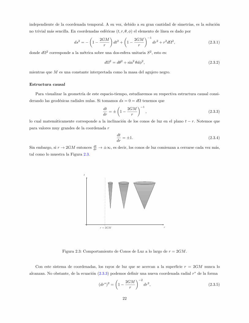
lo cual matematicamente corresponde a la inclinacion de los conos de luz en el plano t − r. Notemos que
para valores muy grandes de la coordenada r
dt
dr= ±1. (2.3.4)
Sin embargo, si r → 2GM entonces dtdr → ±∞, es decir, los conos de luz comienzan a cerrarse cada vez mas,
tal como lo muestra la Figura 2.3.
t
rr = 2GM
Figura 2.3: Comportamiento de Conos de Luz a lo largo de r = 2GM .
Con este sistema de coordenadas, los rayos de luz que se acercan a la superficie r = 2GM nunca lo
alcanzan. No obstante, de la ecuacion (2.3.3) podemos definir una nueva coordenada radial r∗ de la forma
(dr∗)2 =
(1− 2GM
r
)−2
dr2, (2.3.5)
22
donde las geodesicas radiales nulas estaran definidas por
t = ±r∗ + constante. (2.3.6)
Integrando (2.3.5) se obtiene la coordenada tortuga r∗
r∗ = r + 2GM log( r
2GM− 1), (2.3.7)
donde a lo largo de la tesis, consideraremos log := ln. En terminos de esta nueva coordenada, la metrica de
Schwarzschild toma la forma
ds2 =
(1− 2GM
r
)(−dt2 + dr∗2
)+ r2dΩ2. (2.3.8)
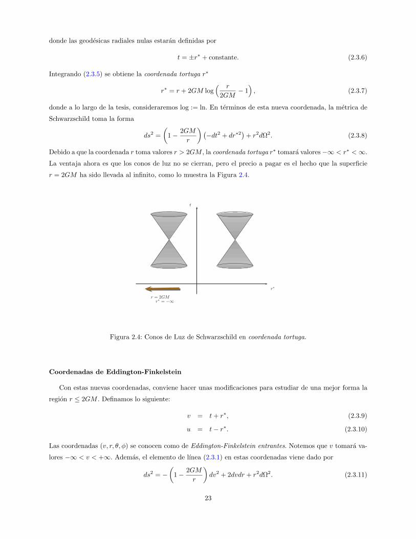
Debido a que la coordenada r toma valores r > 2GM , la coordenada tortuga r∗ tomara valores −∞ < r∗ <∞.
La ventaja ahora es que los conos de luz no se cierran, pero el precio a pagar es el hecho que la superficie
r = 2GM ha sido llevada al infinito, como lo muestra la Figura 2.4.
t
r∗
r = 2GMr∗ = −∞
Figura 2.4: Conos de Luz de Schwarzschild en coordenada tortuga.
Coordenadas de Eddington-Finkelstein
Con estas nuevas coordenadas, conviene hacer unas modificaciones para estudiar de una mejor forma la
region r ≤ 2GM . Definamos lo siguiente:
v = t+ r∗, (2.3.9)
u = t− r∗. (2.3.10)
Las coordenadas (v, r, θ, φ) se conocen como de Eddington-Finkelstein entrantes. Notemos que v tomara va-
lores −∞ < v < +∞. Ademas, el elemento de lınea (2.3.1) en estas coordenadas viene dado por
ds2 = −(
1− 2GM
r
)dv2 + 2dvdr + r2dΩ2. (2.3.11)
23
Es importante notar que en este caso la superficie r = 2GM ya no es singular, debido a que el determinante
de la metrica es g = −r4 sin2 θ y el inverso del tensor metrico existe para este punto. Si consideramos ahora
las geodesicas radiales nulas, obtenemos que
dv
dr=
0 (entrantes),
2
(1− 2GMr )
(salientes).
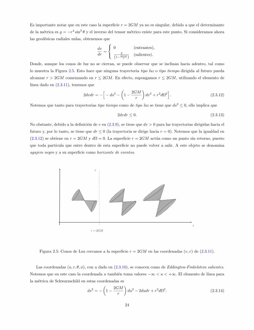
Donde, aunque los conos de luz no se cierran, se puede observar que se inclinan hacia adentro, tal como
lo muestra la Figura 2.5. Esto hace que ninguna trayectoria tipo luz o tipo tiempo dirigida al futuro pueda
alcanzar r > 2GM comenzando en r ≤ 2GM . En efecto, supongamos r ≤ 2GM , utilizando el elemento de
lınea dado en (2.3.11), tenemos que
2dvdr = −[− ds2 −
(1− 2GM
r
)dv2 + r2dΩ2
]. (2.3.12)
Notemos que tanto para trayectorias tipo tiempo como de tipo luz se tiene que ds2 ≤ 0, ello implica que
2dvdr ≤ 0. (2.3.13)
No obstante, debido a la definicion de v en (2.3.9), se tiene que dv > 0 para las trayectorias dirigidas hacia el
futuro y, por lo tanto, se tiene que dr ≤ 0 (la trayectoria se dirige hacia r = 0). Notemos que la igualdad en
(2.3.12) se obtiene en r = 2GM y dΩ = 0. La superficie r = 2GM actua como un punto sin retorno, puesto
que toda partıcula que entre dentro de esta superficie no puede volver a salir. A este objeto se denomina
agujero negro y a su superficie como horizonte de eventos.
r
r = 2GM
v
Figura 2.5: Conos de Luz cercanos a la superficie r = 2GM en las coordenadas (v, r) de (2.3.11).
Las coordenadas (u, r, θ, φ), con u dado en (2.3.10), se conocen como de Eddington-Finkelstein salientes.
Notemos que en este caso la coordenada u tambien toma valores −∞ < u < +∞. El elemento de lınea para
la metrica de Schwarzschild en estas coordenadas es
ds2 = −(
1− 2GM
r
)du2 − 2dudr + r2dΩ2. (2.3.14)
24

Analogo al caso anterior, r = 2GM es no singularidad y el tensor inverso de la metrica en ese punto existe, es
por ello que se puede extender el analisis para r > 0. En estas coordenadas, a diferencia de las de Eddington-
Finkelstein entrantes, los conos de luz se inclinan hacia afuera, tal como lo muestra la Figura 2.6. En este
caso se puede cruzar el horizonte, pero considerando solamente trayectorias dirigidas hacia el pasado, por lo
que ninguna trayectoria tipo luz o tipo tiempo dirigida hacia el futuro puede alcanzar r < 2GM comenzando
en r ≥ 2GM . En efecto, la idea es realizar un procedimiento similar al caso anterior, para r ≤ 2GM
2dudr = −ds2 −(
1− 2GM
r
)du2 + r2dΩ2, (2.3.15)
y si consideramos trayectorias tipo luz o tipo tiempo se tiene ds2 ≤ 0, es decir
2dudr ≥ 0. (2.3.16)
Debido a (2.3.10), para trayectorias dirigidas hacia el futuro se tiene du > 0, obteniendose dr ≥ 0. Por lo
tanto, cualquier partıcula que se encuentre en r < 2GM se dirigira hacia la region exterior. A este objeto se
le conoce como agujero blanco y puede ser considerado como el inverso temporal de un agujero negro.
r
r = 2GM
u
Figura 2.6: Conos de Luz cercanos a la superficie r = 2GM en las coordenadas (u, r) de (2.3.14)
Coordenadas de Kruskal
De las coordenadas de Eddington-Finkelstein, tanto entrantes como salientes, se ha progresado bastante
respecto al analisis de la solucion de Schwarzschild. A continuacion daremos a conocer sistemas de coordena-
das que cubren completamente las regiones de esta solucion. Comencemos el estudio escribiendo la metrica
de Schwarzschild en las coordenadas (u, v, θ, φ)
ds2 = −(
1− 2GM
r
)dudv + r2dΩ2, (2.3.17)
donde r esta definido implıcitamente en terminos de v y u por
1
2(v − u) = r + 2GM log
( r
2GM− 1). (2.3.18)
25

No obstante, notemos que guv se anula en la superficie r = 2GM y, de acuerdo a la ecuacion (2.3.18), tenemos
que v = −∞ o u = +∞. Por este motivo, se realizara un cambio de coordenadas que traiga esta superficie
a una distancia finita. Uno de los posibles cambios corresponde a realizar
V = ev
4GM , (2.3.19)
U = −e− u4GM , (2.3.20)
y en terminos de las coordenadas (V,U, θ, φ) la metrica queda
ds2 = −32G3M3
re−
r2GM dUdV + r2dΩ2, (2.3.21)
donde r queda definida de la forma
UV = −( r
2GM− 1)e
r2GM . (2.3.22)
Debido a la definicion de estas coordenadas, la metrica inicial para la cual r > 2GM hace que el rango
de estas nuevas coordenadas sean U < 0 y V > 0. Notemos ademas que en (2.3.21) no existe problema en
r = 2GM y, por lo tanto, podemos extenderla a los casos U > 0 y V < 0. De esta manera, podemos realizar
un diagrama donde las coordenadas U y V se dibujan a un angulo de 45, como lo muestra la Figura 2.7.
Adicionalmente, de la ecuacion (2.3.22), tenemos que las curvas r constante corresponden a las hiperbolas
UV = constante, mientras que la superficie r = 2GM corresponde al conjunto UV = 0 y la singularidad
r = 0 corresponde a las hiperbolas UV = 1. Por motivos de simplicidad, se ha suprimido las coordenadas
angulares (θ, φ) y, por lo tanto, cada punto de la Figura 2.7 corresponde a una 2-esfera. Como podemos ver,
la figura tiene cuatro regiones claramente definidas. La region I es la variedad de Schwarzschild inicial donde
U < 0 y V > 0. Al extender U > 0 obtenemos la region II, donde su interior corresponde a un agujero
negro. Notemos que si una partıcula entra en la region II, no podra regresar a la region I y el punto de no
retorno U = 0 (r = 2GM) se denomina horizonte de eventos futuro. Asimismo, cualquier trayectoria tipo
tiempo dirigida hacia el futuro que ingrese a la region, termina en la singularidad r = 0. Ademas de estas
dos regiones, en el diagrama aparecen dos regiones adicionales al realizar la continuacion analıtica V < 0. La
region III corresponde al inverso temporal de la region II, el cual es denominado agujero blanco, donde la
superficie V = 0 se denomina horizonte de eventos pasado y es lo que nos separa de este agujero. Por ultimo,
la region IV esta desconectada causalmente de I y corresponde a su inverso temporal.
Consideremos ahora un nuevo sistema en funcion de las coordenadas U y V con tal de obtener una
coordenada tipo tiempo y que el resto de ellas sean tipo espacio:
T =1
2(U + V ) , (2.3.23)
R =1
2(V − U) , (2.3.24)
o en terminos de sus coordenadas originales
T =( r
2GM− 1)1/2
er
4GM sinh
(t
4GM
), (2.3.25)
R =( r
2GM− 1)1/2
er
4GM cosh
(t
4GM
), (2.3.26)
26

III
IVIII
VU
V > 0U < 0
r < 2GM
r > 2GM
r=2GM
r=2G
M
r = 0
r = 0
Figura 2.7: Diagrama de Kruskal.
donde la metrica toma la forma
ds2 =32G3M3
re−
r2GM
(−dT 2 + dR2
)+ r2dΩ2, (2.3.27)
con r definido de manera implıcita como
T 2 −R2 =(
1− r
2GM
)e
r2GM . (2.3.28)
En estas coordenadas, las curvas radiales nulas estan dadas por la relacion
T = ±R+ constante, (2.3.29)
y la superficie r = 2GM corresponde a
T = ±R. (2.3.30)
De la ecuacion (2.3.28), las superficies para r = constante corresponden a las hiperbolas
T 2 −R2 = constante, (2.3.31)
mientras que las superficies con t constante corresponden a las lıneas rectas
T
R= tanh
(t
4GM
). (2.3.32)
Esquematicamente, todo lo anterior se muestra en la Figura 2.8. En la literatura, las coordenadas (T,R, θ, φ)
son conocidas como coordenadas de Kruskal.
27

r = 0
r = 0
r = 2GMt = −∞
r = 2GMt = +∞
r = constante
R
T
t = constante
Figura 2.8: Diagrama de Kruskal en coordenadas T,R.
Diagrama de Carter Penrose
Con las coordenadas de Kruskal se ha recopilado una gran cantidad de informacion respecto a la metrica
de Schwarzschild. Sin embargo, el infinito todavıa se encuentra fuera de la variedad. Ahora el objetivo es
encontrar una transformacion que permita obtener toda la variedad en una region compacta, adicionando
los puntos del infinito. Matematicamente esta transformacion se conoce como compactificacion conforme y
corresponde a realizar
ds2 → ds2 = ω2 (xµ) ds2, (2.3.33)
donde la funcion ω es no nula y debe cumplir la condicion ω → 0 cuando tenemos infinito espacial(xi)→∞
o infinito temporal t =(x0)→ ∞. Como primer ejemplo, consideraremos la variedad de Minkowski. En
coordenadas polares, este espacio-tiempo viene dado por
ds2 = −dt2 + dr2 + r2dΩ2, (2.3.34)
con
−∞ < t < +∞, 0 ≤ r < +∞. (2.3.35)
Realizando el siguiente cambio de coordenadas
u = t− r, v = t+ r, (2.3.36)
tenemos que el nuevo elemento de lınea es el siguiente
ds2 = −dudv +1
4(v − u)2dΩ2, (2.3.37)
y los rangos de estas nuevas coordenadas son
−∞ < u, v < +∞, (2.3.38)
28

con v ≥ u, pues tenemos que r = v−u2 ≥ 0. Ahora, notemos que tanto u como v tienen un rango que
comprende de −∞ a ∞. El siguiente paso es realizar un cambio de coordenadas que transporte el infinito a
un valor finito. La eleccion para este cambio es
u = tanU, v = tanV, (2.3.39)
donde ahora los rangos son
− π
2< U, V <
π
2, (2.3.40)
sujeto a V ≥ U . Con estas nuevas coordenadas (U, V, θ, φ), el elemento de lınea (2.3.37) puede escribirse
como
ds2 =1
(2 cosU cosV )2
[−4 dUdV + sin2(V − U)dΩ2
]. (2.3.41)
De la ecuacion (2.3.41), es natural elegir
ω = 2 cosU cosV. (2.3.42)
Realizando el lımite |U | → π2 o |V | → π
2 , tenemos que ω → 0, es decir, cuando se va a infinito en las
coordenadas iniciales (t, r, θ, φ). Con lo anterior, podemos definir la metrica compactificada de la forma
ds2 = ω2ds2 = −4 dUdV + sin2(V − U)dΩ2. (2.3.43)
Finalmente, realizando un cambio de coordenadas
η = U + V, χ = V − U, (2.3.44)
tenemos que sus respectivos rangos, de acuerdo a (2.3.40), estan dados por
− π < η < π, 0 ≤ χ < π, (2.3.45)
donde el elemento de lınea correspondiente es el siguiente
ds2 = ω2ds2 = −dη2 + dχ2 + sin2 χdΩ2, (2.3.46)
con
ω2 = cos η + cosχ. (2.3.47)
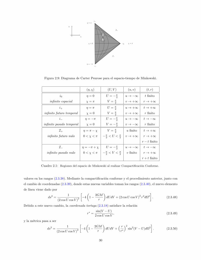
Si suprimimos las coordenadas angulares, obtenemos el respectivo diagrama de Carter Penrose tal como se
observa en la Figura 2.9, el cual consiste en un triangulo que representa la variedad de Minkowski junto
con los puntos de su infinito conforme, que corresponden a la frontera del diagrama, donde cada punto
corresponde a una 2-esfera.
Notemos que en el diagrama anterior, luego de agregar el infinito al espacio-tiempo de Minkowski, existen
cinco regiones claramente definidas, las cuales se explican en el Cuadro 2.1. Ademas, observemos que todas
las trayectorias tipo tiempo comienzan en i− y terminan en i+, mientras que las geodesicas radiales nulas
comienzan en I− y terminan en I+ viajando a 45. Ademas, todas las geodesicas tipo espacio comienzan y
terminan en i0.
Luego de realizar la compactificacion conforme en la variedad de Minkowski, podemos estudiar un analisis
similar considerando la solucion de Schwarzschild y la metrica dada en (2.3.17), donde las coordenadas toman
29
η
χ
i+
i−
i0χ = 0 χ = π
I+
I−
η = π
η = −π
Figura 2.9: Diagrama de Carter Penrose para el espacio-tiempo de Minkowski.
(η, χ) (U, V ) (u, v) (t, r)
i0 η = 0 U = −π2 u→ −∞ t finito
infinito espacial χ = π V = π2 v → +∞ r → +∞
i+ η = π U = π2 u→ +∞ t→ +∞
infinito futuro temporal χ = 0 V = π2 v → +∞ r finito
i− η = −π U = −π2 u→ −∞ t→ −∞infinito pasado temporal χ = 0 V = −π2 v → −∞ r finito
I+ η = π − χ V = π2 u finito t→ +∞
infinito futuro nulo 0 < χ < π −π2 < U < π2 v → +∞ r → +∞
r − t finito
I− η = −π + χ U = −π2 u→ −∞ t→ −∞infinito pasado nulo 0 < χ < π −π2 < V < π
2 v finito r → +∞r + t finito
Cuadro 2.1: Regiones del espacio de Minkowski al realizar Compactificacion Conforme.
valores en los rangos (2.3.38). Mediante la compactificacion conforme y el procedimiento anterior, junto con
el cambio de coordenadas (2.3.39), donde estas nuevas variables toman los rangos (2.3.40), el nuevo elemento
de lınea viene dado por
ds2 =1
(2 cosU cosV )2
[−4
(1− 2GM
r
)dUdV + (2 cosU cosV )
2r2dΩ2
]. (2.3.48)
Debido a este nuevo cambio, la coordenada tortuga (2.3.18) satisface la relacion
r∗ =sin(V − U)
2 cosU cosV, (2.3.49)
y la metrica pasa a ser
ds2 =1
(2 cosU cosV )2
[−4
(1− 2GM
r
)dUdV +
( rr∗
)2
sin2(V − U)dΩ2
]. (2.3.50)
30
Finalmente, tenemos que
ds2 = ω2ds2 = −4
(1− 2GM
r
)dUdV +
( rr∗
)2
sin2(V − U)dΩ2, (2.3.51)
con
ω = 2 cosU cosV, (2.3.52)
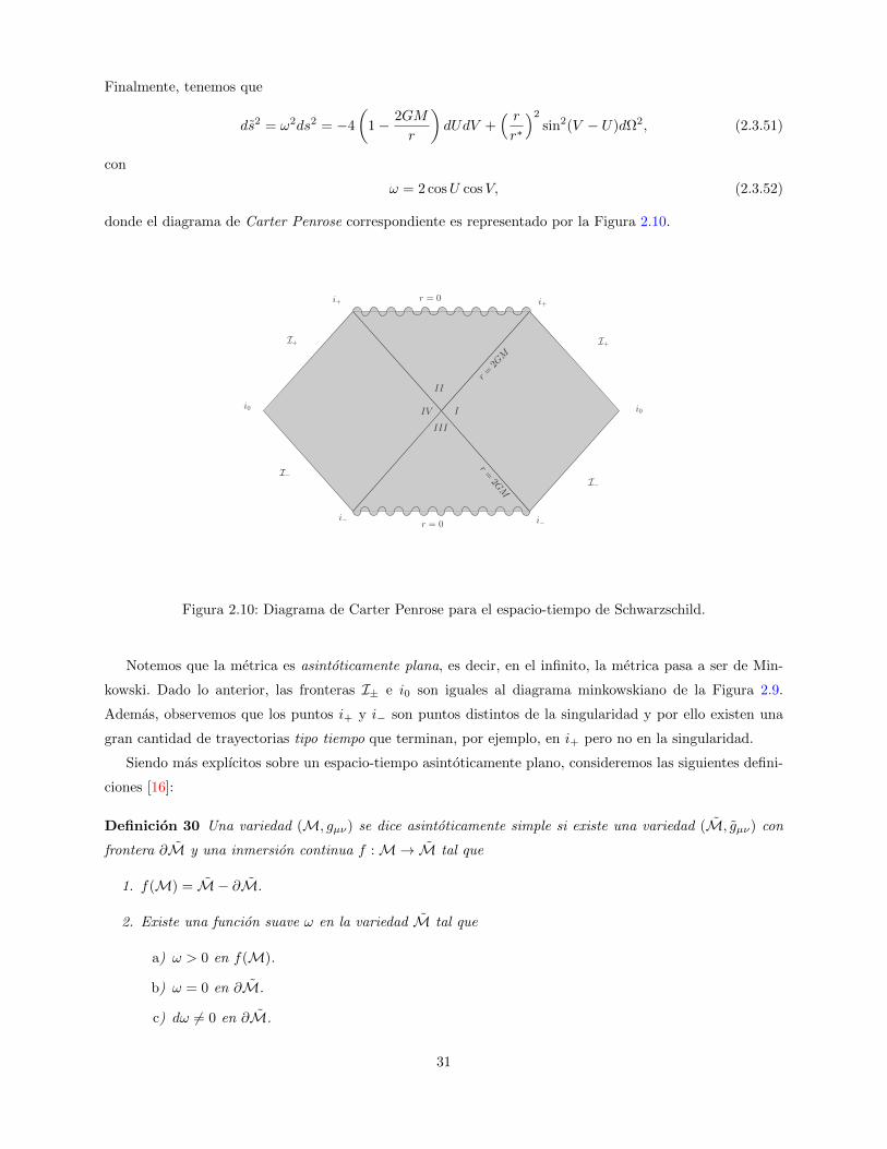
donde el diagrama de Carter Penrose correspondiente es representado por la Figura 2.10.
i+
i−
i0
I+
I−
r = 0
r = 0
i+
i−
I+
i0
I−
II
I
III
IV
r=2GM
r=2GM
Figura 2.10: Diagrama de Carter Penrose para el espacio-tiempo de Schwarzschild.
Notemos que la metrica es asintoticamente plana, es decir, en el infinito, la metrica pasa a ser de Min-
kowski. Dado lo anterior, las fronteras I± e i0 son iguales al diagrama minkowskiano de la Figura 2.9.
Ademas, observemos que los puntos i+ y i− son puntos distintos de la singularidad y por ello existen una
gran cantidad de trayectorias tipo tiempo que terminan, por ejemplo, en i+ pero no en la singularidad.
Siendo mas explıcitos sobre un espacio-tiempo asintoticamente plano, consideremos las siguientes defini-
ciones [16]:
Definicion 30 Una variedad (M, gµν) se dice asintoticamente simple si existe una variedad (M, gµν) con
frontera ∂M y una inmersion continua f :M→ M tal que
1. f(M) = M − ∂M.
2. Existe una funcion suave ω en la variedad M tal que
a) ω > 0 en f(M).
b) ω = 0 en ∂M.
c) dω 6= 0 en ∂M.
31
d) Satisface gµν = ω2gµν .
3. Toda geodesica nula en la variedad M tiene dos puntos extremos en ∂M.
Definicion 31 Una variedad (M, gµν) se denomina debil asintoticamente simple si existe un abierto U ⊂Mque sea isometrico a una vecindad abierta de ∂M, donde M corresponde a la compactificacion conforme de
alguna variedad asintoticamente simple.
Definicion 32 Una variedad se denomina asintoticamente vacıa si Rµν = 0 en alguna vecindad abierta de
∂M, donde M es la compactificacion conforme de alguna variedad asintoticamente simple.
Definicion 33 Una variedad se denomina asintoticamente plana si es debil asintoticamente simple y asintoti-
camente vacıa.
2.3.2. Agujero negro de Reissner-Nordstrom
A continuacion estudiaremos soluciones que representan agujeros negros cargados electricamente. De las
ecuaciones de Einstein (2.2.3), tenemos que el tensor de energıa-momento Tµν de la accion
− 1
4
∫d4x√−gFµνFµν , (2.3.53)
es dado por
Tµν = FµσFσ
ν −1
4gµνFσρF
σρ, (2.3.54)
donde Fµν = ∂µAν − ∂νAµ corresponde al tensor electromagnetico y Aµ se conoce como vector potencial.
Adicionalmente, al variar la accion respecto a ∂µAν tenemos
∇µFµν = 0. (2.3.55)
Dado que estamos enfocados en una solucion con simetrıa esferica y con campo electrico, de la ecuacion
(2.3.55) tenemos que tensor Fµν adquiere la forma
Frt =Q
r2, (2.3.56)
donde la constante de integracion Q correspondera a la carga electrica. El objetivo ahora es encontrar la
metrica de un agujero negro cargado electricamente tal que se reduzca a la solucion de Schwarzschild cuando
la carga sea nula. La solucion es conocida usualmente como la metrica de Reissner-Nordstrom [17, 18]
ds2 = −(
1− 2GM
r+GQ2
r2
)dt2 +
(1− 2GM
r+GQ2
r2
)−1
dr2 + r2dΩ2, (2.3.57)
donde podemos reescribir el elemento de lınea de la forma
ds2 = −∆
r2dt2 +
r2
∆dr2 + r2dΩ2, (2.3.58)
con
∆ = r2 − 2GMr +GQ2. (2.3.59)
32
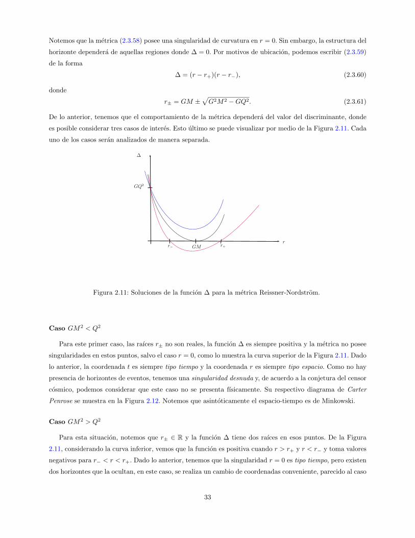
Notemos que la metrica (2.3.58) posee una singularidad de curvatura en r = 0. Sin embargo, la estructura del
horizonte dependera de aquellas regiones donde ∆ = 0. Por motivos de ubicacion, podemos escribir (2.3.59)
de la forma
∆ = (r − r+)(r − r−), (2.3.60)
donde
r± = GM ±√G2M2 −GQ2. (2.3.61)
De lo anterior, tenemos que el comportamiento de la metrica dependera del valor del discriminante, donde
es posible considerar tres casos de interes. Esto ultimo se puede visualizar por medio de la Figura 2.11. Cada
uno de los casos seran analizados de manera separada.
∆
r
GQ2
r− r+GM
Figura 2.11: Soluciones de la funcion ∆ para la metrica Reissner-Nordstrom.
Caso GM2 < Q2
Para este primer caso, las raıces r± no son reales, la funcion ∆ es siempre positiva y la metrica no posee
singularidades en estos puntos, salvo el caso r = 0, como lo muestra la curva superior de la Figura 2.11. Dado
lo anterior, la coordenada t es siempre tipo tiempo y la coordenada r es siempre tipo espacio. Como no hay
presencia de horizontes de eventos, tenemos una singularidad desnuda y, de acuerdo a la conjetura del censor
cosmico, podemos considerar que este caso no se presenta fısicamente. Su respectivo diagrama de Carter
Penrose se muestra en la Figura 2.12. Notemos que asintoticamente el espacio-tiempo es de Minkowski.
Caso GM2 > Q2
Para esta situacion, notemos que r± ∈ R y la funcion ∆ tiene dos raıces en esos puntos. De la Figura
2.11, considerando la curva inferior, vemos que la funcion es positiva cuando r > r+ y r < r− y toma valores
negativos para r− < r < r+. Dado lo anterior, tenemos que la singularidad r = 0 es tipo tiempo, pero existen
dos horizontes que la ocultan, en este caso, se realiza un cambio de coordenadas conveniente, parecido al caso
33

i+
i−
i0
I+
I−
r = 0
Figura 2.12: Diagrama de Carter Penrose considerando GM2 < Q2.
de Schwarzschild. Su respectivo diagrama de Penrose se grafica en la Figura 2.13, donde podemos diferenciar
dos regiones claramente definidas, esquematizadas por medio de dos cuadros. El primero de ellos (el cuadro
inferior) contiene una singularidad esencial en r = 0, donde se observa que esta no es asintoticamente plana.
Sin embargo, la segunda region (cuadro superior) posee una estructura igual a la de Minkowski en la frontera.
Adicionalmente, podemos apreciar que cada una de estas dos regiones se repiten de manera infinita, es por
eso que solo se expuso un estracto del diagrama de Carter Penrose, donde el comportamiento de cada una
de estas regiones depende de los valores de r±.
Un fenomeno interesante ocurre en la Figura 2.13, el cual se representa por medio de una flecha. Supon-
gamos que un observador comienza en la region la cual corresponde a la base de la flecha y cae hacia el
horizonte r = r+, cuando lo cruza, observamos que la coordenada temporal se vuelve tipo espacio, mientras
que la coordenada espacial se vuelve tipo tiempo. Sin embargo, cuando cruza el horizonte r = r−, ocurre
un intercambio nuevamente entre las coordenadas espaciales y temporales, y la caıda hacia la singularidad
r = 0 puede evitarse, cruzando nuevamente el horizonte r = r−, donde el observador es forzado a moverse
para cruzar finalmente el horizonte r = r+, esquematizado mediante la punta de la flecha. Lo anterior lo
podemos interpretar como un infinito numero de regiones asintoticamente planas conectadas por tuneles de
agujeros negros.
Caso GM2 = Q2
El ultimo caso a considerar es cuando el discriminante de la funcion ∆ es nulo, esto es
∆ = (r − r+)(r − r−) = (r −GM)2. (2.3.62)
Particularmente, tenemos que la metrica de Reissner-Nordstrom es dada por
ds2 = −(
1− GM
r
)2
dt2 +
(1− GM
r
)−2
dr2 + r2dΩ2. (2.3.63)
34
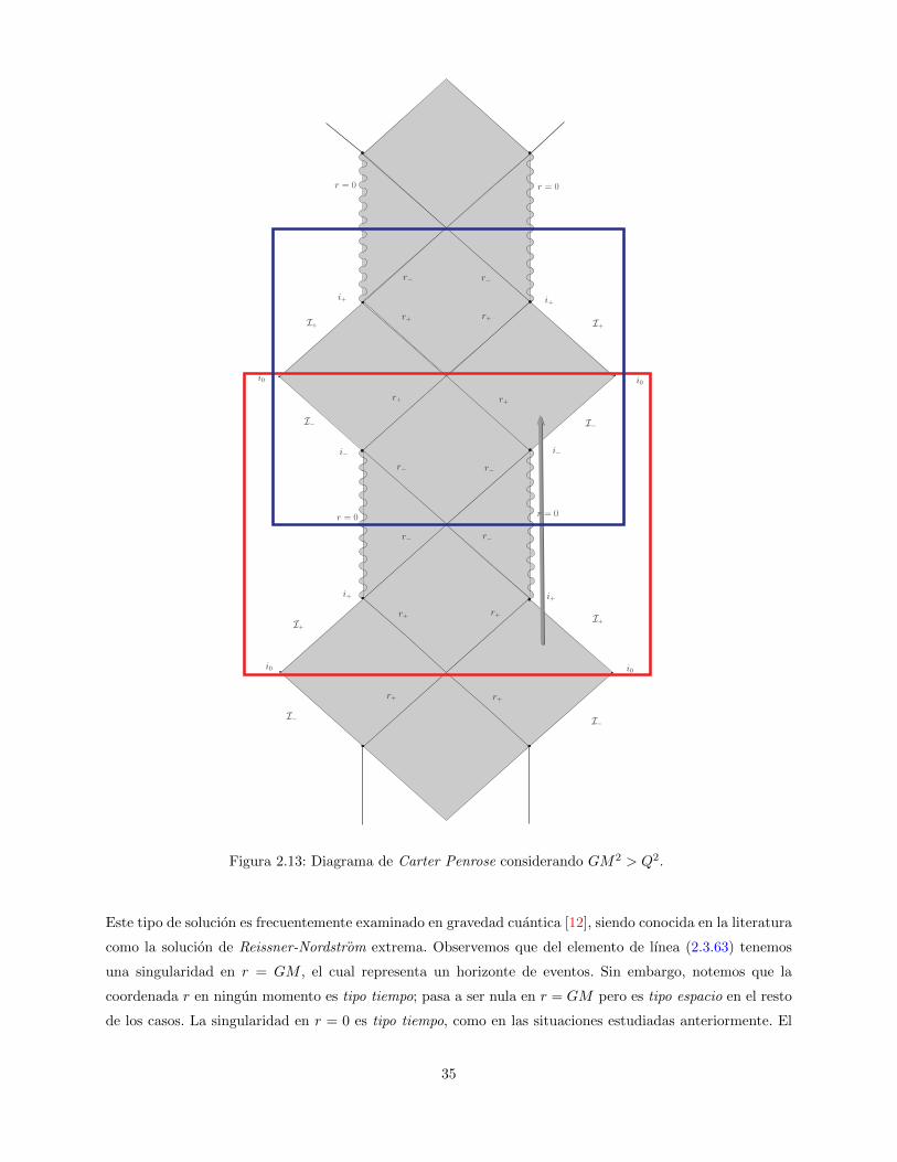
i+
r = 0r = 0
i+
I+
i−
r− r−
r+ r+
r+ r+
r− r−
r− r−
r+ r+
r+ r+
i+
I+I+
I−I−
i−
i+
i0i0
r = 0r = 0
i0i0
I+
I− I−
Figura 2.13: Diagrama de Carter Penrose considerando GM2 > Q2.
Este tipo de solucion es frecuentemente examinado en gravedad cuantica [12], siendo conocida en la literatura
como la solucion de Reissner-Nordstrom extrema. Observemos que del elemento de lınea (2.3.63) tenemos
una singularidad en r = GM , el cual representa un horizonte de eventos. Sin embargo, notemos que la
coordenada r en ningun momento es tipo tiempo; pasa a ser nula en r = GM pero es tipo espacio en el resto
de los casos. La singularidad en r = 0 es tipo tiempo, como en las situaciones estudiadas anteriormente. El
35

r = 0
I−
i0
I+
I+
i0
i0
I−r = 0
i+
i−
r =GM
r =GM
r =∞
r=∞
Figura 2.14: Diagrama de Carter Penrose considerando GM2 = Q2.
diagrama de Carter Penrose, esquematizado en la Figura 2.14, es similar al caso GM2 > Q2, con la diferencia
que ahora la singularidad se encuentra siempre a la izquierda.
2.3.3. Agujero negro de Kerr
Aunque las soluciones de Schwarzschild y Reissner-Nordstrom fueron descubiertas poco tiempo despues
de la Relatividad General de Einstein, solo en el ano de 1963 se encontro una solucion para agujeros negros
36
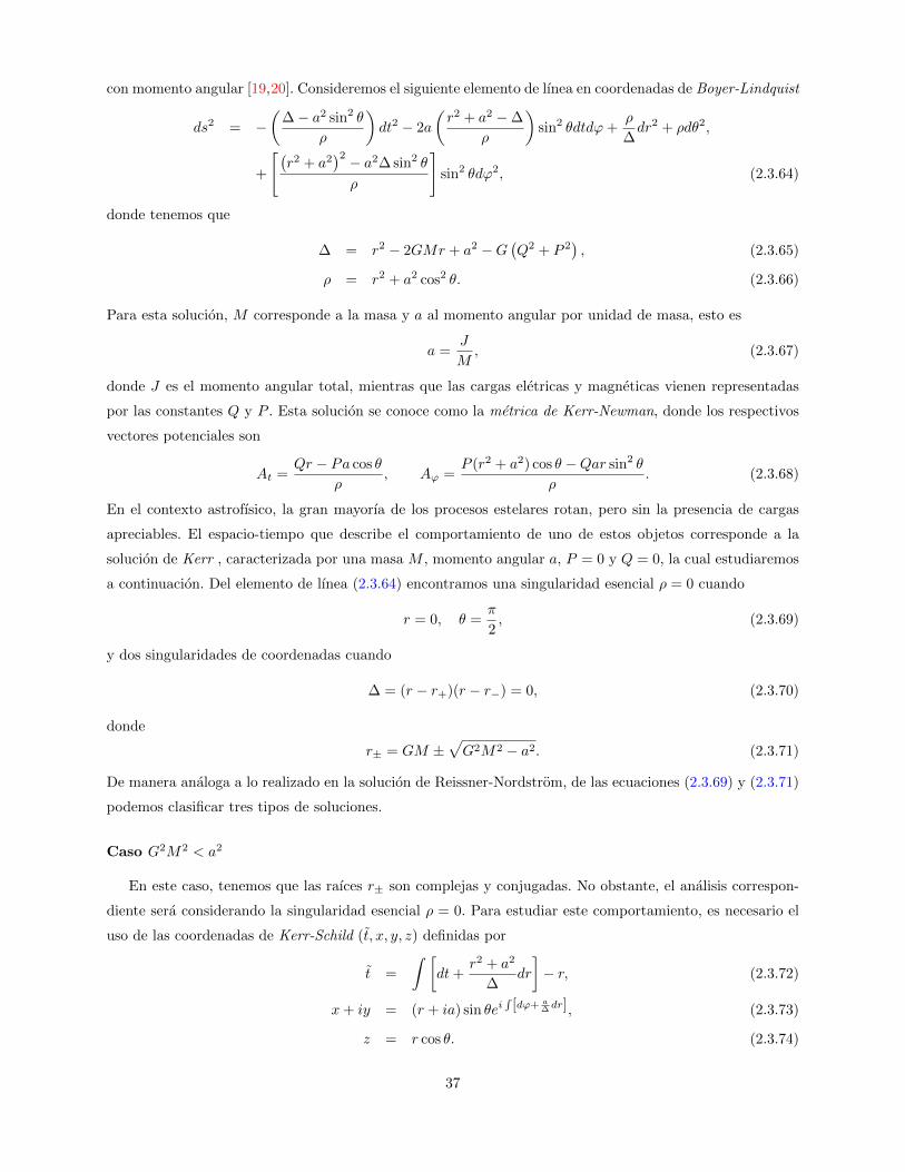
con momento angular [19,20]. Consideremos el siguiente elemento de lınea en coordenadas de Boyer-Lindquist
ds2 = −(
∆− a2 sin2 θ
ρ
)dt2 − 2a
(r2 + a2 −∆
ρ
)sin2 θdtdϕ+
ρ
∆dr2 + ρdθ2,
+
[(r2 + a2
)2 − a2∆ sin2 θ
ρ
]sin2 θdϕ2, (2.3.64)
donde tenemos que
∆ = r2 − 2GMr + a2 −G(Q2 + P 2
), (2.3.65)
ρ = r2 + a2 cos2 θ. (2.3.66)
Para esta solucion, M corresponde a la masa y a al momento angular por unidad de masa, esto es
a =J
M, (2.3.67)
donde J es el momento angular total, mientras que las cargas eletricas y magneticas vienen representadas
por las constantes Q y P . Esta solucion se conoce como la metrica de Kerr-Newman, donde los respectivos
vectores potenciales son
At =Qr − Pa cos θ
ρ, Aϕ =
P (r2 + a2) cos θ −Qar sin2 θ
ρ. (2.3.68)
En el contexto astrofısico, la gran mayorıa de los procesos estelares rotan, pero sin la presencia de cargas
apreciables. El espacio-tiempo que describe el comportamiento de uno de estos objetos corresponde a la
solucion de Kerr , caracterizada por una masa M , momento angular a, P = 0 y Q = 0, la cual estudiaremos
a continuacion. Del elemento de lınea (2.3.64) encontramos una singularidad esencial ρ = 0 cuando
r = 0, θ =π
2, (2.3.69)
y dos singularidades de coordenadas cuando
∆ = (r − r+)(r − r−) = 0, (2.3.70)
donde
r± = GM ±√G2M2 − a2. (2.3.71)
De manera analoga a lo realizado en la solucion de Reissner-Nordstrom, de las ecuaciones (2.3.69) y (2.3.71)
podemos clasificar tres tipos de soluciones.
Caso G2M2 < a2
En este caso, tenemos que las raıces r± son complejas y conjugadas. No obstante, el analisis correspon-
diente sera considerando la singularidad esencial ρ = 0. Para estudiar este comportamiento, es necesario el
uso de las coordenadas de Kerr-Schild (t, x, y, z) definidas por
t =
∫ [dt+
r2 + a2
∆dr
]− r, (2.3.72)
x+ iy = (r + ia) sin θei∫[dϕ+ a
∆dr], (2.3.73)
z = r cos θ. (2.3.74)
37
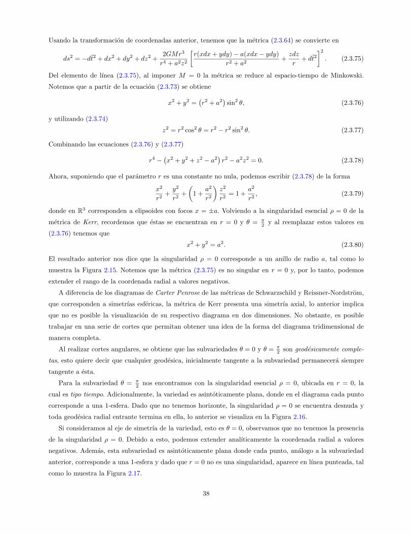
Usando la transformacion de coordenadas anterior, tenemos que la metrica (2.3.64) se convierte en
ds2 = −dt2 + dx2 + dy2 + dz2 +2GMr3
r4 + a2z2
[r(xdx+ ydy)− a(xdx− ydy)
r2 + a2+zdz
r+ dt2
]2
. (2.3.75)
Del elemento de lınea (2.3.75), al imponer M = 0 la metrica se reduce al espacio-tiempo de Minkowski.
Notemos que a partir de la ecuacion (2.3.73) se obtiene
x2 + y2 =(r2 + a2
)sin2 θ, (2.3.76)
y utilizando (2.3.74)
z2 = r2 cos2 θ = r2 − r2 sin2 θ. (2.3.77)
Combinando las ecuaciones (2.3.76) y (2.3.77)
r4 −(x2 + y2 + z2 − a2
)r2 − a2z2 = 0. (2.3.78)
Ahora, suponiendo que el parametro r es una constante no nula, podemos escribir (2.3.78) de la forma
x2
r2+y2
r2+
(1 +
a2
r2
)z2
r2= 1 +
a2
r2, (2.3.79)
donde en R3 corresponden a elipsoides con focos x = ±a. Volviendo a la singularidad esencial ρ = 0 de la
metrica de Kerr, recordemos que estas se encuentran en r = 0 y θ = π2 y al reemplazar estos valores en
(2.3.76) tenemos que
x2 + y2 = a2. (2.3.80)
El resultado anterior nos dice que la singularidad ρ = 0 corresponde a un anillo de radio a, tal como lo
muestra la Figura 2.15. Notemos que la metrica (2.3.75) es no singular en r = 0 y, por lo tanto, podemos
extender el rango de la coordenada radial a valores negativos.
A diferencia de los diagramas de Carter Penrose de las metricas de Schwarzschild y Reissner-Nordstrom,
que corresponden a simetrıas esfericas, la metrica de Kerr presenta una simetrıa axial, lo anterior implica
que no es posible la visualizacion de su respectivo diagrama en dos dimensiones. No obstante, es posible
trabajar en una serie de cortes que permitan obtener una idea de la forma del diagrama tridimensional de
manera completa.
Al realizar cortes angulares, se obtiene que las subvariedades θ = 0 y θ = π2 son geodesicamente comple-
tas, esto quiere decir que cualquier geodesica, inicialmente tangente a la subvariedad permanecera siempre
tangente a esta.
Para la subvariedad θ = π2 nos encontramos con la singularidad esencial ρ = 0, ubicada en r = 0, la
cual es tipo tiempo. Adicionalmente, la variedad es asintoticamente plana, donde en el diagrama cada punto
corresponde a una 1-esfera. Dado que no tenemos horizonte, la singularidad ρ = 0 se encuentra desnuda y
toda geodesica radial entrante termina en ella, lo anterior se visualiza en la Figura 2.16.
Si consideramos al eje de simetrıa de la variedad, esto es θ = 0, observamos que no tenemos la presencia
de la singularidad ρ = 0. Debido a esto, podemos extender analıticamente la coordenada radial a valores
negativos. Ademas, esta subvariedad es asintoticamente plana donde cada punto, analogo a la subvariedad
anterior, corresponde a una 1-esfera y dado que r = 0 no es una singularidad, aparece en lınea punteada, tal
como lo muestra la Figura 2.17.
38

z
x−a a
Superficies con r constante
ϕθ
Figura 2.15: Superficies con r constante y singularidad esencial ρ = 0.
i+
i−
r = 0 i0
I+
I−
Figura 2.16: Diagrama de Carter Penrose considerando θ = π2 y la singularidad ρ = 0.
Caso G2M2 > a2
El segundo caso a considerar es cuando tenemos dos raıces reales en (2.3.71), las cuales corresponden a
singularidades de coordenadas, junto con la singularidad esencial ρ = 0. Notemos que la funcion ∆ es positiva
39
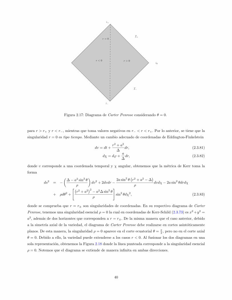
i+
i−
i0
I+
I−
r = 0
r > 0r < 0
Figura 2.17: Diagrama de Carter Penrose considerando θ = 0.
para r > r+ y r < r−, mientras que toma valores negativos en r− < r < r+. Por lo anterior, se tiene que la
singularidad r = 0 es tipo tiempo. Mediante un cambio adecuado de coordenadas de Eddington-Finkelstein
dv = dt+r2 + a2
∆dr, (2.3.81)
dχ = dϕ+a
∆dr, (2.3.82)
donde v corresponde a una coordenada temporal y χ angular, obtenemos que la metrica de Kerr toma la
forma
ds2 = −(
∆− a2 sin2 θ
ρ
)dv2 + 2dvdr − 2a sin2 θ
(r2 + a2 −∆
)
ρdvdχ− 2a sin2 θdrdχ
+ ρdθ2 +
[(r2 + a2
)2 − a2∆ sin2 θ
ρ
]sin2 θdχ2, (2.3.83)
donde se comprueba que r = r± son singularidades de coordenadas. En su respectivo diagrama de Carter
Penrose, tenemos una singularidad esencial ρ = 0 la cual en coordenadas de Kerr-Schild (2.3.73) es x2 +y2 =
a2, ademas de dos horizontes que corresponden a r = r±. De la misma manera que el caso anterior, debido
a la simetrıa axial de la variedad, el diagrama de Carter Penrose debe realizarse en cortes asintoticamente
planos. De esta manera, la singularidad ρ = 0 aparece en el corte ecuatorial θ = π2 , pero no en el corte axial
θ = 0. Debido a ello, la variedad puede extenderse a los casos r < 0. Al fusionar los dos diagramas en una
sola representacion, obtenemos la Figura 2.18 donde la lınea punteada corresponde a la singularidad esencial
ρ = 0. Notemos que el diagrama se extiende de manera infinita en ambas direcciones.
40

Caso G2M2 = a2
El ultimo caso a estudiar corresponde a la metrica de Kerr extrema, esto es cuando
∆ = (r − r−)(r − r+) = (r −GM)2, (2.3.84)
donde su respectivo diagrama de Carter Penrose esta dado por la Figura 2.19. Observemos que la region
asintoticamente plana se conecta con la region que posee la singularidad ρ = 0, la cual en coordenadas de
Kerr-Schild (2.3.73) corresponde a x2 + y2 = a2. Ademas, la region completa, la cual se extiende de manera
infinita en ambas direcciones, esta compuesta por el corte ecuatorial θ = π2 , el cual posee la singularidad
esencial ρ = 0, y el corte axial θ = 0. Es importante notar que esta singularidad es tipo tiempo, siendo
representada mediante una lınea punteada.
41

i+i+
I+
r+ r+
r+ r+
r− r−
r+ r+
r+ r+
I+
I−
i0
i0
I+
I−
I−
r = 0r = 0
r− r−
r = 0r = 0
I+
I−
r− r−
i−i−
i+i+
i−i−
i−i−
Figura 2.18: Diagrama de Carter Penrose considerando G2M2 > a2.
42
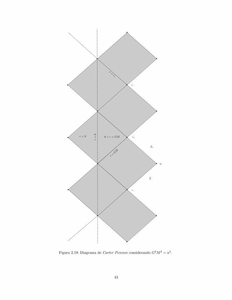
r=
0
i+
i−
i−
r < 0 0 < r < GM
r =GM
b
b
b
b
b
b
b
bb
bb
bb
b b
b
i0
r =r+
I+
I−
Figura 2.19: Diagrama de Carter Penrose considerando G2M2 = a2.
43

Capıtulo 3
Agujeros negros en presencia de un
campo escalar no mınimamente
acoplado a la curvatura escalar
En la actualidad, teorıas cuanticas de campos (TCC) fuertemente acopladas son problemas difıciles de
resolver en fısica teorica. Sin embargo, hace 16 anos se propuso una importante correspondencia entre la TCC
y teorıas gravitatorias, las cuales incluyen la Relatividad General de Einstein y su generalizacion en Teorıa
de Cuerdas [21–23], permitiendo encontrar nuevas direcciones que logren enlazar la Mecanica Cuantica con
la gravedad [24].
En muchas aplicaciones, como por ejemplo en fısica de altas energıas y teorıa de cuerdas, se estudian TCC
invariantes bajo transformaciones conformes, estas son aquellas invariantes bajo escalamiento, las transfor-
maciones de Lorentz y las traslaciones de la teorıa de la Relatividad Especial. Todas estas transformaciones
forman el llamado grupo conforme y el espacio dual con la simetrıa apropiada para esta invariancia co-
rresponde al espacio-tiempo anti-de Sitter (AdS) [24], es por este motivo que en la literatura es conocida
comunmente como correspondencia AdS/CFT (anti-de Sitter/Teorıa de Campos Conforme) (ver por ejem-
plo la resena [25]). A modo de introduccion, comenzaremos nuestro estudio dando a conocer las variedades
simetricas maximales, las cuales son aquellas cuya curvatura es la misma en todas partes, ası como tambien
en todas direcciones. Para estos casos, tenemos que el tensor de Riemann en estos ambientes en dimension
D, con una metrica gµν , es de la forma
Rρσµν = K(gρµgσν − gρνgσµ), (3.0.1)
donde K corresponde a una medida normalizada de la curvatura escalar [12]
K =R
D(D − 1). (3.0.2)
Ahora, tomando la traza del tensor de Riemann dado en (3.0.1), obtenemos una expresion para el tensor de
44

Ricci en D-dimensiones, el cual es proporcional a la metrica gµν :
Rµν = K(D − 1)gµν . (3.0.3)
De lo anterior, podemos clasificar tres espacio-tiempos maximalmente simetricos, el primero de ellos co-
rresponde al de Minkowski, donde su curvatura es cero en todas partes (K = 0). Si K > 0 obtenemos el
espacio-tiempo de Sitter (dSD), mientras que si K < 0 tenemos anti-de Sitter (AdSD).
Por otra parte, consideremos las ecuaciones de Einstein en el vacıo con una constante cosmologica Λ [26],
esto es
Gµν + Λgµν = 0. (3.0.4)
Si tomamos la traza de (3.0.4) obtenemos que
R =2D
(D − 2)Λ. (3.0.5)
Reemplazando (3.0.5) en (3.0.4) obtenemos una relacion entre el tensor de Ricci y la constante cosmologica
dada por
Rµν =2Λ
(D − 2)gµν , (3.0.6)
donde el signo de Λ clasifica cada uno de estos tres espacio-tiempos expuestos anteriormente. Si Λ = 0
obtenemos el caso de Minkowski, si Λ > 0 tenemos el caso dSD y si Λ < 0 tendremos AdSD.
Recordemos que para las soluciones de Schwarzchild y Reissner-Nordstrom, estudiadas en el capıtulo 2, la
topologıa del horizonte es esferica, y son respaldadas por los teoremas de Hawking e Israel [27–29]. Mas aun,
para un espacio-tiempo de dimension cuatro existen ciertos teoremas de censura topologica que restringen
posibles geometrıas de agujeros negros [30]. De lo anterior, cabe preguntarse si es posible encontrar otras
configuraciones de tal manera de eludir estos teoremas. Una manera es trabajar en dimensiones superiores
a cuatro, donde en [31] encuentran una solucion cuya topologıa del horizonte no es esferica, conocida como
anillo negro. Otra forma es considerar a la gravedad de Einstein una constante cosmologica, encontrando
agujeros negros con horizontes no esfericos en dimension cuatro [32–34], ası como tambien extensiones para
dimensiones superiores [35]. Estas soluciones se conocen como agujeros negros topologicos.
Considerar teorıas en las cuales tenemos una fuente de materia son, en estricto rigor, un problema no
trivial, debido basicamente a la conjetura del no-pelo (no-hair conjeture) [36] enunciado originalmente por
John Archibald Wheller, inspirado por los teoremas de unicidad de las soluciones de Schwarzchild, Reissner-
Nordstrom, Kerr y Kerr-Newman [28,29,37–39], postulando que todas las soluciones de agujeros negros en las
ecuaciones de Einstein-Maxwell de gravitacion y electromagnetismo pueden ser caracterizadas solamente por
tres parametros observables de manera externa, correspondientes a la masa, carga y momento angular (ver por
ejemplo la resena [40]). Sin embargo, en la decada de 1970, los trabajos realizados por Bocharova, Bronnikov
y Melnikov [41], y posteriormente por Bekenstein [42], mostraron que un campo escalar no mınimamente
acoplado resulta un buen laboratorio en orden de evadir esta conjetura. Mas aun, estas teorıas sostienen una
solucion de agujero negro conocida como la solucion BBMB (Bocharova-Bronnikov-Melnikov-Bekenstein),
donde a lo largo de los anos ha sido el pilar fundamental para nuevas soluciones que involucran un campo
escalar con acoplamiento no minimal.
45
El plan de este capıtulo esta organizado como sigue. En la proxima seccion se estudian soluciones conside-
rando la accion gravitatoria de Einstein-Hilbert en presencia de un campo escalar no mınimamente acoplado
conforme, explicando algunas soluciones clasicas presentes en la literatura, ademas de la inclusion de dos
3-formas no trivialmente acopladas al campo escalar, logrando ası extender el caso conforme. En la seccion
3.2 se considera un caso particular de una teorıa gravitatoria conocida como gravedad de Lovelock, siendo
la extension mas natural de la Relatividad General considerando un espacio-tiempo de dimension superior,
donde las ecuaciones de movimiento son a lo mas de segundo orden. Finalmente, en las seccion 3.3 se exponen
los resultados presentes en [1, 2].
3.1. Agujeros negros en presencia de un campo escalar no mıni-
mamente acoplado a la curvatura escalar conforme
Formalmente, consideremos la siguiente accion de materia en D-dimensiones
SM[gµν ,Φ] =1
2
∫ √−gdDx[∂µΦ∂µΦ + ξRΦ2
], (3.1.1)
donde ξ es conocido como constante de acoplamiento no minimal y R es la curvatura escalar. Es importante
notar que cuando la constante de acoplamiento no minimal ξ desaparece (ξ = 0), tenemos el caso de un
campo escalar mınimamente acoplado. Para una constante ξ de la forma
ξD =D − 2
4 (D − 1), (3.1.2)
la accion (3.1.1) es invariante conforme, esto quiere decir que bajo las transformaciones
gµν 7→ Ω2 gµν , Φ 7→ Ω−(D−2)/2 Φ, (3.1.3)
se tiene que
SM[gµν ,Φ] = SM[gµν , Φ] + terminos de frontera, (3.1.4)
donde Ω es una funcion diferenciable y estrictamente positiva.
Si variamos la accion (3.1.1) respecto a la metrica, ası como tambien respecto al campo escalar Φ, tenemos
Tµν = ∇µΦ∇νΦ− gµν(
1
2∇σΦ∇σΦ
)+ ξ(gµν−∇µ∇ν +Gµν)Φ2, (3.1.5)
Φ = ξRΦ, (3.1.6)
donde := gµν∇µ∇ν y para una constante de acoplamiento no minimal de la forma (3.1.2), se obtiene que
Tµµ = gµνTµν = 0. Si consideramos una teorıa de gravedad acoplada a un campo escalar no mınimamente
acoplado en D dimensiones, esto es
S =1
2κ
∫dDx√−gR− SM[gµν ,Φ], (3.1.7)
al variar la accion respecto al campo escalar obtenemos la ecuacion (3.1.6), mientras que variando la accion
respecto a la metrica gµν tenemos
Gµν = κTµν . (3.1.8)
46
Aquı, Tµν es el tensor de energıa-momento calculado previamente en (3.1.5). Si calculamos la traza de (3.1.8),
podemos concluir que para este tipo de teorıas la curvatura escalar R se desvanece. Una solucion de agujero
negro a estas ecuaciones de movimiento, la cual es estatica con simetrıa esferica, junto con un campo escalar
de la forma
Φ = Φ(r),
es la solucion BBMB [41,42], la cual en dimension cuatro, con ξ = ξ4 = 16 , viene dada por
ds2 = −(
1− M
r
)2
dt2 +
(1− M
r
)−2
dr2 + r2(dθ2 + sin2 θdφ2
), (3.1.9)
Φ(r) =
√6
κ
M
r −M . (3.1.10)
De la solucion (3.1.9) podemos concluir que esta solucion es asintoticamente plana. Mas aun, Xanthopoulos
y Zannias estudian la solucion mas general para una solucion estatica, asintoticamente plana, con simetrıa
esferica de las ecuaciones de Einstein acoplada a un campo escalar conforme, demostrando que la unica
solucion de agujero negro corresponde a la solucion BBMB [43]. Ademas, en [44] analizan la teorıa para una
dimension D arbitraria, encontrando soluciones para el caso conforme acoplado y extendiendo el metodo de
transformacion elaborado por Bekenstein por medio de soluciones mınimamente acopladas [42], mostrando
que la solucion de agujero negro BBMB solamente existe en dimension cuatro. Sin embargo, a pesar de estos
resultados, la deficiencia de esta solucion esta en el hecho que el campo escalar Φ diverge en el horizonte de
eventos, haciendo su interpretacion fısica y el problema de su estabilidad un problema de debate [45,46]. Una
manera de eludir este problema de divergencia es a traves de la inclusion de una constante cosmologica a las
ecuaciones de movimiento, donde la divergencia del campo escalar ocurre dentro del horizonte de eventos.
Concretamente, en [47] consideran una teorıa de gravedad con una constante cosmologica no negativa, donde
ademas del acoplamiento conforme del campo escalar se incluye un potencial U(Φ) dado por
U(Φ) = αΦ4, (3.1.11)
donde α corresponde a una constante, manteniendo la invariancia conforme del campo escalar. La teorıa es
presentada de la siguiente manera
SMTZ =1
16πG
∫d4x√−g(R− 2Λ)− SM[gµν ,Φ]− α
∫d4x√−gΦ4, (3.1.12)
con ξ = ξ4 = 16 y hemos reemplazado κ por 8πG. Las ecuaciones de movimiento al variar respecto a la
metrica gµν y al campo escalar Φ son
Gµν + Λgµν = 8πG[Tµν − αgµνΦ4
], (3.1.13)
Φ = ξRΦ + 4αΦ3. (3.1.14)
Debido a la invariancia conforme de la seccion asociada a la fuente de materia, la traza del nuevo tensor
de energıa momento tambien es nula, lo cual implica que, a diferencia de la solucion BBMB, la curvatura
escalar es una constante cuyo valor es
R = 4Λ, (3.1.15)
47

y la solucion, conocida en la literatura como agujero negro MTZ, viene dada por el elemento de lınea
ds2 = −[−r
2
l2+
(1− GM
r
)2]dt2 +
[−r
2
l2+
(1− GM
r
)2]−1
dr2 + r2(dθ2 + sin2 θdφ2
), (3.1.16)
junto a un campo escalar
Φ(r) =
√3G
4π
M
r −GM , (3.1.17)
mientras que el potential adquiere la forma
U(Φ) = − 2
3l2πGΦ4, (3.1.18)
y la constante cosmologica se expresa como
Λ =3
l2, (3.1.19)
donde l corresponde al radio cosmologico [47] y r ∈ [0,+∞). Notemos que para esta solucion, el horizonte
de eventos se encuentra en
rh =l
2
(1 +
√1− 4GM
l
), (3.1.20)
donde M corresponde a una constante de integracion asociada al parametro de masa, con GM ∈(0, l4).
Adicionalmente, vemos que
0 < GM < rh, (3.1.21)
donde podemos observar que la divergencia del campo escalar Φ se encuentra en una region al interior del
horizonte. Asimismo, en [47] estudian soluciones de agujero negro cargados electricamente, esto es adicionar
a la accion (3.1.12)
− 1
16π
∫d4x√−gFµνFµν , (3.1.22)
donde la componente no nula del tensor de Maxwell es
Frt = −Ftr = ∂rAt =Q
r2. (3.1.23)
Aquı, Q es una constante de integracion asociada a la carga. Reemplazando en las ecuaciones de movimiento,
podemos notar una restriccion entre la masa M y la carga Q dada por
Q2 = M2G
(1 +
2πG
3αl2
), (3.1.24)
donde la constante cosmologica Λ (3.1.19) y el elemento de lınea (3.1.16) mantienen su estructura. Ademas,
el parametro α debe satisfacer
α < −2πG
3l2, (3.1.25)
mientras que el campo escalar Φ toma la forma
Φ(r) =
√− 1
2αl2GM
r −GM . (3.1.26)
48
En el ano 2006, Martınez, Staforelli y Troncoso [48] extienden este resultado por medio del siguiente
ansatz metrico
ds2 = −F (r)dt2 +dr2
F (r)+ r2dσ2
γ , (3.1.27)
donde dσ2γ representa el elemento de lınea de una variedad base 2-dimensional Σ , la cual asumen compacta,
sin frontera y con curvatura constante asociada al parametro γ, con γ = −1, 0,+1. Mientras que la teorıa
a estudiar corresponde a la accion (3.1.12) junto con (3.1.22). Una de las cosas interesantes de esta nueva
solucion, esta en el hecho que tanto la funcion metrica F (r) como la relacion entre los parametros de masa
M y carga Q dependen de la constante γ, esto es
F (r) = −Λr2
3+ γ
(1 +
GM
r
)2
, Q2 = γM2
(1 +
2πΛG
9α
), (3.1.28)
mientras que el campo escalar adquiere la forma
Φ(r) =
√− Λ
6α
GM
r +GM, (3.1.29)
y el tensor de Maxwell es como (3.1.23).
Para γ = 1 logran reproducir la solucion encontrada en [47] para una constante cosmologica Λ no negativa.
Si consideramos un horizonte hiperbolico (γ = −1), la constante cosmologica es negativa, siendo
Λ = − 3
l2, (3.1.30)
donde la solucion posee una singularidad de curvatura en r = 0. Debido a esta estructura topologica, los
autores separan el analisis en tres casos dependiendo del signo de la masa M , la cual para valores positivos
se tiene que el horizonte de eventos se encuentra localizado en
rh =l
2
(1 +
√1 +
4GM
l
). (3.1.31)
Aquı el campo escalar Φ y el tensor de Maxwell son dados por (3.1.29) y (3.1.23) respectivamente, y α ∈(0, 2πG
3l2
]. Si la masa es nula, tenemos que tanto el campo escalar como el campo electromagnetico desaparecen,
produciendo una metrica de la forma
ds2 = −(r2
l2− 1
)dt2 +
(r2
l2− 1
)−1
dr2 + r2dσ2−1. (3.1.32)
Sin embargo, para una masa M negativa acotada en − l4G ≤M < 0, el agujero negro posee tres horizontes,
donde los autores lo catalogan como un agujero negro dentro de un agujero negro [48]. El horizonte mas
externo viene dado por (3.1.31), el cual rodea a la singularidad del campo escalar ubicada en r = −GM .
Para soluciones cuyo horizonte de eventos es planar (γ = 0), el campo electromagnetico se desvanece, la
constante cosmologica es de la forma (3.1.30) y la metrica es dada por
ds2 = −r2
l2dt2 +
l2
r2dr2 + r2dσ2
0 , (3.1.33)
la cual corresponde al espacio-tiempo anti-de Sitter (AdS). Ademas, la masa desaparece y la constante de
integracion M es interpretada como un pelo en el campo escalar Φ, el cual mantiene la estructura estudiada
49

previamente en (3.1.29), ası como tambien para el potencial (3.1.11). Cabe destacar que este tipo de soluciones
son conocidas como configuraciones stealth, esto es una solucion no trivial donde
Gµν + Λgµν = 0 = 8πG[Tµν − αgµνΦ4
]. (3.1.34)
Es decir, son soluciones en las cuales tanto la parte materia como la parte gravedad se desvanecen identica-
mente (ver por ejemplo la referencia [49], donde estudian estas clases de configuraciones en tres dimensiones).
Adicionalmente, en [50] los autores encuentran nuevas clases de soluciones en dimension cuatro considerando
un potencial de la forma
U(Φ) = −Λ√
6κ
9
χ
χ2 + 1
[− 6
κΦ + Φ3
]− κΛ
36Φ4, (3.1.35)
donde χ es un parametro arbitrario, Λ es la constante cosmologica y κ = 8πG. Concretamente, las ecuaciones
de movimiento son
Gµν + Λgµν = κ [Tµν − gµνU(Φ)] , Φ = ξRΦ +dU
dΦ, (3.1.36)
y, como antes, ξ = ξ4. Dado lo precedente, tenemos que la solucion adquiere la forma
ds2 =
(r + (χ− 1)M
)2
(r −M)2
−
(γ(
1− M
r
)2
− λr2
3
)dt2 +
dr2
(γ(
1− Mr
)2
− λr2
3
) + r2dσ2γ
,(3.1.37)
Φ(r) =
(6
κ
)1/2M (χ− 1)− χrr +M (χ− 1)
, (3.1.38)
λ =Λ(χ2 − 1
)2
χ2 + 1, (3.1.39)
donde ahora el elemento de lınea dσγ solo puede tomar valores γ = ±1. Dependiendo del signo de la constante
cosmologica Λ, ası como tambien de la eleccion del parametro γ, se logran clasificar nuevas clases de soluciones
exactas. Por ejemplo, los casos Λ > 0, γ = 1 y Λ < 0, γ = −1 resultan soluciones de agujeros negros [50].
3.1.1. Agujeros negros en presencia de (D − 1)-formas
Dados los resultados anteriores en dimension cuatro, podemos observar que solamente se encuentran
soluciones de agujeros negros considerando un acoplamiento no minimal conforme (3.1.2), ası como tambien
un horizonte esferico o hiperbolico. Una manera de encontrar configuraciones planares a las ecuaciones de
Einstein, considerando un ansatz metrico (3.1.27) con γ = 0, es adicionar a la accion (3.1.12) dos 3-formas
no trivialmente acopladas al campo escalar Φ [51,52], esto es
Saxionic = −∫d4x√−g
[ε(Φ)
12
2∑
i=1
H(i)α1α2α3
H(i)α1α2α3
], (3.1.40)
50

junto con el termino de Maxwell (3.1.22) y ξ = ξ4 = 16 . Las ecuaciones de movimiento respecto a los diferentes
campos dinamicos son de la forma
Gµν + Λgµν = 8πG[Tµν − gµνU(Φ) + TMaxwell
µν + T axionic
µν
], (3.1.41)
Φ = ξRΦ +dU
dΦ+dε
dΦ
[1
12
2∑
i=1
H(i)α1α2α3
H(i)α1α2α3
], (3.1.42)
∂α
(√−g ε(Φ)H(i)αα1···αD−2
)= 0, ∂α
(√−gFαβ)
= 0, (3.1.43)
donde
T axionic
µν = ε(Φ)
2∑
i=1
[1
2H(i)µα1α2
H(i)α1α2ν − gµν
12H(i)α1α2α3
H(i)α1α2α3
], (3.1.44)
TMaxwell
µν =1
4π
[FµσF
σν − gµνFαβFαβ
], (3.1.45)
mientras que el potencial U(Φ) es como (3.1.11). Para una constante cosmologica de la forma (3.1.30), la
solucion es dada por [52]
ds2 = −[r2
l2− p2
(1 +
Gµ
r
)2]dt2 +
[r2
l2− p2
(1 +
Gµ
r
)2]−1
dr2 + r2(dx2
1 + dx22
),
Φ(r) =1√2αl
Gµ
r +Gµ, H(i) = − p√
8πG
(1− 4πG
3Φ2
)dt ∧ dr ∧ dxi,
F = − q
r2dt ∧ dr, (3.1.46)
mientras que las constantes satisfacen la relacion
q2 = p2µ2G
(2πG
3αl2− 1
). (3.1.47)
La caracterıstica mas importante de este resultado es el hecho que corresponde a la version planar del agujero
negro MTZ [47] expuesto al principio de esta seccion. Del mismo modo, manteniendo la esencia explicada con
anterioridad, en [53] encuentran agujeros negros para una constante de acoplamiento no minimal ξ arbitraria,
siendo uno de los primeros ejemplos para esta clase de configuraciones. Concretamente, para una constante
ξ 6= 14 y un potencial U(Φ) de la forma
U(Φ) =Φ2
8πGl2
[3ξ(1− 6ξ) +
2ξ2
(1− 4ξ)2
(2 (1− 6ξ) + bΦ
1−4ξ2ξ
)2], (3.1.48)
complementado por una funcion ε(Φ)
ε(Φ) =
(1− 8πGξΦ2
)
f(√
8πGΦ), (3.1.49)
donde
f(Φ) = ξ2Φ1−2ξξ
[16ξΣ2Φ
4ξ−12ξ − Σ1
(1
1− 4ξ− ξΦ2
)]
+ (1− 4ξ)
[(1− 6ξ) (1− ξΦ2) + 2ξ
(1− ξ
1− 4ξΦ2
)], (3.1.50)
51
y una constante cosmologica dada por (3.1.30), la teorıa admite una solucion de la forma
ds2 = −F (r) dt2 +1
F (r)dr2 +
r2
l2(dx2
1 + dx22
), Φ(r) =
1√8πG
(ar + b)−2ξ1−4ξ ,
H(i) =p√
8πG (1− 4ξ)2l2ε(Φ)
dt ∧ dr ∧ dxi, F = − q
r2dt ∧ dr, (3.1.51)
donde la funcion F (r) y la constante a son dadas por
F (r) =r2
l2− p2 (ar + b)
4ξ1−4ξ
(ar + b)4ξ
1−4ξ − ξ
(1 +
2Gµ
r− Gq2
p2r2
), a =
1
Gµ(b− Σ2) , (3.1.52)
mientras que el resto de las constantes estan sujetas a la restriccion
q2 =p2µ2G
(b− Σ2)2
(2bΣ2 − b2 −
Σ1
2 (1− 4ξ)
). (3.1.53)
Por otro lado, tomando el valor particular ξ = 14 tanto el potencial U(Φ) como la funcion ε(Φ) adquieren
la expresion
U(Φ) =Φ2
32πGl2
(2 log
(Φ
b
)2
+ 6 log
(Φ
b
)+ 3
), (3.1.54)
ε(Φ) =
(8πGΦ2 − 4
)2
f(√
8πGΦ), (3.1.55)
donde b es una constante y la funcion f(Φ) es dada por
f(Φ) = 2Φ2 log
(Φ
b
)(4 log
(Φ
b
)− Φ2
)+ 4
(Φ2 − 4
)+ Σ1Φ2
[8 log
(Φ
b
)−(Φ2 − 4
)]. (3.1.56)
Finalmente, la solucion es
ds2 = −F (r) dt2 +1
F (r)dr2 +
r2
l2(dx2
1 + dx22
), Φ(r) =
1√8πG
bear,
H(i) =p
4√
8πG l2ε(Φ)dt ∧ dr ∧ dxi, F = 0, (3.1.57)
donde
F (r) =r2
l2− p2
(b2e2ar − 4)
(1 +
µ
r
), a =
Σ1 − 1
µ. (3.1.58)
Notemos que para este valor especial de la constante ξ, no es factible acomodar un campo de Maxwell cargado
electricamente. Adicionalmente a lo anterior, los autores en [53] extienden la version en D-dimensiones donde
ahora la teorıa corresponde a la inclusion de (D − 2) campos, los cuales corresponden a (D − 1)-formas
acopladas por una funcion ε(Φ), esto es
Saxionic
D = −∫dDx√−g
[ε(Φ)
2 (D − 1)!
D−2∑
i=1
H(i)α1···αD−1H(i)α1···αD−1
]. (3.1.59)
3.2. Gravedad de Lovelock
La extension mas general de la accion de Einstein-Hilbert en dimension cuatro esta dada por el Lagran-
giano
52
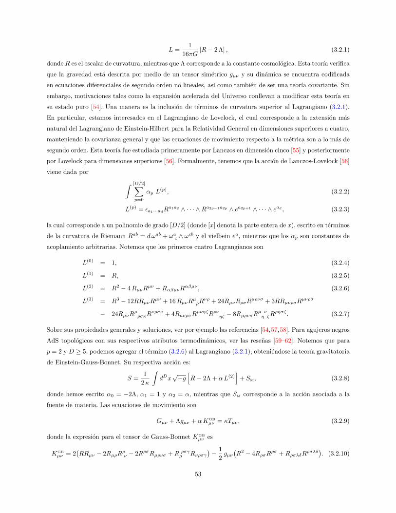
L =1
16πG[R− 2 Λ] , (3.2.1)
donde R es el escalar de curvatura, mientras que Λ corresponde a la constante cosmologica. Esta teorıa verifica
que la gravedad esta descrita por medio de un tensor simetrico gµν y su dinamica se encuentra codificada
en ecuaciones diferenciales de segundo orden no lineales, ası como tambien de ser una teorıa covariante. Sin
embargo, motivaciones tales como la expansion acelerada del Universo conllevan a modificar esta teorıa en
su estado puro [54]. Una manera es la inclusion de terminos de curvatura superior al Lagrangiano (3.2.1).
En particular, estamos interesados en el Lagrangiano de Lovelock, el cual corresponde a la extension mas
natural del Lagrangiano de Einstein-Hilbert para la Relatividad General en dimensiones superiores a cuatro,
manteniendo la covarianza general y que las ecuaciones de movimiento respecto a la metrica son a lo mas de
segundo orden. Esta teorıa fue estudiada primeramente por Lanczos en dimension cinco [55] y posteriormente
por Lovelock para dimensiones superiores [56]. Formalmente, tenemos que la accion de Lanczos-Lovelock [56]
viene dada por
∫ [D/2]∑
p=0
αp L(p), (3.2.2)
L(p) = εa1···adRa1a2 ∧ · · · ∧Ra2p−1a2p ∧ ea2p+1 ∧ · · · ∧ ead , (3.2.3)
la cual corresponde a un polinomio de grado [D/2] (donde [x] denota la parte entera de x), escrito en terminos
de la curvatura de Riemann Rab = dωab + ωac ∧ ωcb y el vielbein ea, mientras que los αp son constantes de
acoplamiento arbitrarias. Notemos que los primeros cuatro Lagrangianos son
L(0) = 1, (3.2.4)
L(1) = R, (3.2.5)
L(2) = R2 − 4RµνRµν +RαβµνR
αβµν , (3.2.6)
L(3) = R3 − 12RRµνRµν + 16RµνR
µρR
νρ + 24RµνRρσRµρνσ + 3RRµνρσR
µνρσ
− 24RµνRµρσκR
νρσκ + 4RµνρσRµνηζRρσηζ − 8RµρνσR
µ νη ζR
ρησζ . (3.2.7)
Sobre sus propiedades generales y soluciones, ver por ejemplo las referencias [54,57,58]. Para agujeros negros
AdS topologicos con sus respectivos atributos termodinamicos, ver las resenas [59–62]. Notemos que para
p = 2 y D ≥ 5, podemos agregar el termino (3.2.6) al Lagrangiano (3.2.1), obteniendose la teorıa gravitatoria
de Einstein-Gauss-Bonnet. Su respectiva accion es:
S =1
2κ
∫dDx√−g
[R− 2Λ + αL(2)
]+ SM, (3.2.8)
donde hemos escrito α0 = −2Λ, α1 = 1 y α2 = α, mientras que SM corresponde a la accion asociada a la
fuente de materia. Las ecuaciones de movimiento son
Gµν + Λgµν + αKGB
µν = κTµν , (3.2.9)
donde la expresion para el tensor de Gauss-Bonnet KGBµν es
KGB
µν = 2(RRµν − 2RµρR
ρν − 2RρσRµρνσ +R ρσγ
µ Rνρσγ)− 1
2gµν(R2 − 4RρσR
ρσ +RρσλδRρσλδ
). (3.2.10)
53

A lo largo de los anos, se han presentado una gran cantidad de soluciones considerando esta clase de teorıa,
las primeras de ellas fueron encontradas por Boulware y Deser [63], e independientemente por Wheeler [64].
Posteriormente, se considero un campo electromagnetico [65] y en los anos siguientes se estudiaron las
propiedades termodinamicas para agujeros negros AdS topologicos dada una constante cosmologica negativa
[66].
Como lo muestra [61], para que la teorıa (3.2.2) posea un unico vacıo de AdS, fijando la constante
cosmologica, se debe restringir las constantes de acoplamiento αp, obteniendose un conjunto de teorıas
indexadas por un entero k de la forma
Ik = − 1
2k(D − 3)!
∫ k∑
p=0
Ckp(D − 2p)
L(p), 1 ≤ k ≤[D − 1
2
], (3.2.11)
donde Ckp corresponde a un factor combinatorial. Mas aun, podemos reescribir la accion (3.2.11) como
Ik =1
2κ
∫dDx√−g
[R+
(D − 1)(D − 2)
k+
(k − 1)
2(D − 3)(D − 4)L(2)
+(k − 1)(k − 2)
3!(D − 3)(D − 4)(D − 5)(D − 6)L(3) + · · ·
]. (3.2.12)
De manera mas precisa, podemos considerar la accion en D-dimensiones de la forma Sk = Ik + SM, donde,
como antes, SM es la accion correspondiente a la fuente de materia. De lo anterior, las ecuaciones de movi-
miento adquieren la estructura G(k)µν = κTµν , donde G(k)
µν es el tensor gravitatorio asociado a la variacion de
la accion Ik, esto es
G(k)µν = Gµν −
(D − 1)(D − 2)
2kgµν +
(k − 1)
2(D − 3)(D − 4)KGB
µν
+(k − 1)(k − 2)
3!(D − 3)(D − 4)(D − 5)(D − 6)Sµν + · · · . (3.2.13)
Aquı, KGBµν es el tensor de Gauss-Bonnet expuesto en (3.2.10), mientras que Sµν se obtiene variando L(3)
dado en (3.2.7), siendo
Sµν = 3(R2Rµν − 4RRρµR
ρν − 4RρσRρσRµν + 8RρσRρµRσν − 4RRρσRρµσν
+8RρκRσκRρµσν − 16RρσRκ(µR|κσρ|ν) + 2RRρσκµRρσκν +RµνRρσκηRρσκη
−8Rρ(µRσκη|ρ|R|σκη|ν) − 4RρσRκηρµRκησν + 8RρσR
ρκσηRκµην − 8RρσRρκη
µRσκην
+4RρσκηRρσζµRζ
κη ν − 8RρκσηRζρσµRζκην − 4RρσκηRρσκζRη ζµ ν
)− 1
2gµνL
(3). (3.2.14)
3.3. Agujeros negros asintoticamente AdS con horizonte planar
en presencia de un campo escalar no mınimamente acoplado
a la curvatura escalar
En general, para encontrar soluciones de agujeros negros se considera el siguiente ansatz metrico:
ds2γ = −f(r) dt2 +
dr2
g(r)+ r2dΣ2
D−2,γ , (3.3.1)
54

donde dΣ2D−2,γ expresa el elemento de lınea de una esfera (D − 2)-dimensional (γ = 1), un hiperboloide
(γ = −1) o un plano (γ = 0), esto es
dΣ2D−2,γ =
dx2D−2 +
∑D−3k=1
(∏D−2j=k+1 sin2(xj)
)dx2
k para γ = 1,
dx2D−2 +
∑D−3k=1
(∏D−2j=k+1 sinh2(xj)
)dx2
k para γ = −1,
dx2D−2 +
∑D−3k=1 dx
2k para γ = 0.
En particular, se puede mostrar que la solucion general de las ecuaciones de Einstein con constante
cosmologica negativa sin una fuente de materia viene dada por [25,35]
f(r) = g(r) = γ +r2
l2− M
rD−3, Λ = − (D − 1)(D − 2)
2 l2, (3.3.2)
donde M es constante de integracion asociada a la masa y l es el radio AdS. Manteniendo el mismo espıritu,
en [1] se estudian soluciones con una topologıa del horizonte planar (γ = 0), las cuales son asintoticamente
AdS, considerando una teorıa particular de la gravedad de Lovelock, estudiada en la seccion 3.2 (con k = 2),
ademas de un campo escalar no mınimamente acoplado a la curvatura escalar, motivados por tener una mejor
comprension en superconductores no convencionales [67–69]. Posteriormente, en [2] se considera la extension
natural del trabajo anterior en orden de reforzar la idea que estas clases de soluciones estan fuertemente
relacionadas a teorıas gravitatorias con terminos de curvatura superior. Adicionalmente, se muestra que estas
soluciones emergen de una configuracion stealth definidas sobre la metrica (donde hemos impuesto l := 1)
ds20 = −r2dt2 +
dt2
r2+ r2dΣ2
D−2,0. (3.3.3)
Esto es, una solucion no trivial que satisface simultaneamente
G(k)µν = 0 = Tµν ,
donde G(k)µν corresponde a las ecuaciones de movimiento asociadas a la teorıa gravitatoria, mientras que Tµν
es su correspondiente tensor de energıa-momento. De lo anterior, podemos realizar una transformacion de la
metrica (3.3.3) de la forma [13]
gµν = gµν − S kµkν ,
conocida en la literatura como transformacion Kerr-Schild. Para esta expresion, gµν corresponde a la metrica
base (3.3.3), S es una funcion escalar y kµ es un vector nulo respecto a ambas metricas, es decir
kµkµ = gµνkµkν = gµνk
µkν = 0, gµν = gµν + 2Skµkν . (3.3.4)
Lo interesante es que esta combinacion, esto es la configuracion stealth y la transformacion Kerr-Schild,
permite encontrar dos familias de soluciones con un horizonte de eventos planar, las cuales se caracterizan
por un valor particular de la constante de acoplamiento no minimal ξ. Ademas, si agregamos a la teorıa
(D − 1)-formas, logramos extender estos resultados para una constante ξ arbitraria. Cada una de estas
soluciones seran analizadas a continuacion y corresponden a los resultados presentes en los artıculos [1, 2].
55

Topological black holes for Einstein-Gauss-Bonnet gravity with a nonminimal scalar field
Moises Bravo Gaete* and Mokhtar Hassaıne†
Instituto de Matematica y Fısica, Universidad de Talca, Casilla 747, Talca, Chile(Received 27 August 2013; published 12 November 2013)
We consider the Einstein-Gauss-Bonnet gravity with a negative cosmological constant together with a
source given by a scalar field nonminimally coupled in arbitrary dimensionD. For a certain election of the
cosmological and Gauss-Bonnet coupling constants, we derive two classes of AdS black hole solutions
whose horizon is planar. The first family of black holes obtained for a particular value of the nonminimal
coupling parameter only depends on a constant M, and the scalar field vanishes as M ¼ 0. The second
class of solutions corresponds to a two-parametric (with constants M and A) black hole stealth
configuration, which is a nontrivial scalar field with a black hole metric such that both sides (gravity
and matter parts) of the Einstein equations vanish. In this case, in the vanishingM, the solution reduces to
a stealth scalar field on the pure AdS metric. We note that the existence of these two classes of solutions is
indicative of the particular choice of the coupling constants, and they cannot be promoted to spherical or
hyperboloid black hole solutions in a standard fashion. In the last part, we add to the original action some
exact (D 1) forms coupled to the scalar field. The direct benefit of introducing such extra fields is to
obtain black hole solutions with a planar horizon for an arbitrary value of the nonminimal coupling
parameter.
DOI: 10.1103/PhysRevD.88.104011 PACS numbers: 04.50.Gh
I. INTRODUCTION
The anti-de Sitter/conformal field theory (AdS/CFT)correspondence is a power tool that permits us to analyzestrongly coupled systems by mapping them into somehigher-dimensional gravity theories and establishing asort of dictionary between both theories [1]. Recently,these ideas have been extended to nonrelativistic physicsin order to describe certain condensed matter systems (e.g.see [2,3] for recent reviews) or in order to gain a betterunderstanding of some unconventional superconductors[4–6]. In this last case, the minimal ingredients in thegravity side are given by the Einstein-Hilbert action witha negative cosmological constant, together with a chargedself-interacting (complex) scalar field with the Maxwellterm. Moreover, in order to reproduce the superconductorphase diagram, the system must admit black holes withscalar hair at low temperatures, and this hair must disap-pear at high temperatures. However, this problem of find-ing black hole solutions with a scalar field is rendereddifficult by the various no-hair theorems existing in thecurrent literature; see e.g. [7]. Nevertheless, such no-gotheorems can be avoided by considering scalar fields non-minimally coupled to gravity [8,9]. By nonminimallycoupled scalar fields, we mean a scalar field with itsusual kinetic term, together with a term coupled to theRicci scalar R as R2 where is the nonminimal cou-pling parameter. We precisely consider this kind of mattersource in order to escape the traditional no-hair theorems.
For the gravity Lagrangian, we are concerned with theEinstein-Gauss-Bonnet action with a negative cosmologicalconstant. This choice is motivated by the recent interestin holographic superconductors in Einstein-Gauss-Bonnetgravity. Indeed, holographic superconductors in such gravitytheory have been studied intensively with the purpose ofanalyzing the effects of the Gauss-Bonnet coupling constanton the critical temperature and on the condensate; see e.g.[10–12].More specifically, we consider a matter action given by a
particular Einstein-Gauss-Bonnet gravity action, togetherwith a self-interacting scalar field nonminimally coupled togravity, and we look for black holes; for good reviews onEinstein-Gauss-Bonnet black holes, see e.g. [13,14]. For thismodel, we derive two classes of black hole solutions with aplanar base manifold and only for particular values of thenonminimal coupling parameter. Note that the first examplesof topological black holes in general relativity (GR) werediscussed in [15]. In our case, for ¼ ðD 2Þ=ð4DÞ and¼ðD1Þ=ð4Dþ4Þ, we obtain AdS black holes whosemetrics resemble the Schwarzschild-AdS-Tangherlini space-time. In both cases, and in contrast with the Bocharova-Bronnikov-Melnikov-Bekenstein solution [8,9], the scalarfield does not diverge at the horizon. This is due to thepresence of the negative cosmological constant as it occursfor the known black hole solutions with scalar fields in fourdimensions [16–18]. For the first family of solutions, thescalar field depends on the mass constant M and vanishesidentically as M ¼ 0, yielding to the purely AdS solutionwithout a source. The second class of solutions is, to ourknowledge, the first example of a higher-dimensional blackhole stealth configuration. This means a nontrivial scalarfield together with a black hole metric such that both sides
*[email protected]†Corresponding author.
PHYSICAL REVIEW D 88, 104011 (2013)
1550-7998=2013=88(10)=104011(7) 104011-1 2013 American Physical Society
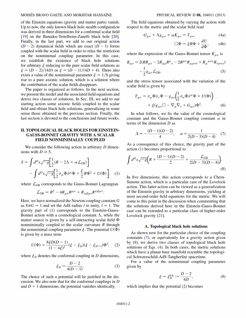
of the Einstein equations (gravity and matter parts) vanish.Up to now, the only known black hole stealth configurationwas derived in three dimensions for a conformal scalar field[19] on the Banados-Teitelboim-Zanelli black hole [20].Finally, in the last part, we add to our original action(D 2) dynamical fields which are exact (D 1) formscoupled with the scalar field in order to relax the restrictionon the nonminimal coupling parameter. In this case,we establish the existence of black hole solutionsfor arbitrary reducing to the pure scalar field solutions as ¼ ðD 2Þ=ð4DÞ or ¼ ðD 1Þ=ð4Dþ 4Þ. There alsoexists a value of the nonminimal parameter ¼ 1=8 givingrise to a pure axionic solution, which is a solution wherethe contribution of the scalar fields disappears.
The paper is organized as follows. In the next section,we present the model and the associated field equations andderive two classes of solutions. In Sec. III, we add to ourstarting action some axionic fields coupled to the scalarfield and obtain black hole solutions, generalizing in somesense those obtained in the previous section. Finally, thelast section is devoted to the conclusions and future works.
II. TOPOLOGICAL BLACKHOLES FOREINSTEIN-GAUSS-BONNET GRAVITY WITH A SCALAR
FIELD NONMINIMALLY COUPLED
We consider the following action in arbitrary D dimen-sions with D 5,
S ¼Z
dDxffiffiffiffiffiffiffig
p 1
2ðR 2þ LGBÞ
Z
dDxffiffiffiffiffiffiffig
p 1
2@@þ
2R2 þUðÞ
; (1)
where LGB corresponds to the Gauss-Bonnet Lagrangian
LGB ¼ R2 4RR þ RR
:
Here, we have normalized the Newton coupling constantGas 8G ¼ 1 and set the AdS radius l to unity, l ¼ 1. Thegravity part of (1) corresponds to the Einstein-Gauss-Bonnet action with a cosmological constant , while thematter source is given by a self-interacting scalar field nonminimally coupled to the scalar curvature R throughthe nonminimal coupling parameter . The potential UðÞis given by a mass term
UðÞ ¼ 8DðD 1Þð1 4Þ2 ð DÞð Dþ1Þ2; (2)
where D denotes the conformal coupling in D dimensions,
D ¼ D 2
4ðD 1Þ : (3)
The choice of such a potential will be justified in the dis-cussion. We also note that for the conformal couplings in Dand Dþ 1 dimensions, the potential vanishes identically.
The field equations obtained by varying the action withrespect to the metric and the scalar field read
G þg þ K ¼ T; (4a)
h ¼ Rþ dU
d; (4b)
where the expression of the Gauss-Bonnet tensor K is
K ¼ 2ðRR 2RR 2RRþR
RÞ 1
2gLGB; (5)
and the stress tensor associated with the variation of thescalar field is given by
T ¼ @@ g
1
2@@þUðÞ
þ ðghrr þGÞ2: (6)
In what follows, we fix the value of the cosmologicalconstant and the Gauss-Bonnet coupling constant interms of the dimension D as
¼ðD1ÞðD2Þ4
; ¼ 1
2ðD3ÞðD4Þ : (7)
As a consequence of this choice, the gravity part of theaction (1) becomes proportional to
ZdDx
ffiffiffiffiffiffiffigp
Rþ ðD 1ÞðD 2Þ2
þ LGB
2ðD 3ÞðD 4Þ:
(8)
In five dimensions, this action corresponds to a Chern-Simons action, which is a particular case of the Lovelockaction. This latter action can be viewed as a generalizationof the Einstein gravity in arbitrary dimensions, yielding atmost second-order field equations for the metric. We willcome to this point in the discussion when commenting thatthe solutions derived here in the Einstein-Gauss-Bonnetcase can be extended to a particular class of higher-orderLovelock gravity [21].
A. Topological black hole solutions
As shown now for the particular choice of the couplingconstants (7), or equivalently for a gravity action givenby (8), we derive two classes of topological black holesolutions of Eqs. (4). In both cases, the metric solutionswhich have a planar base manifold resemble the topologi-cal Schwarzschild-AdS-Tangherlini spacetime.For a value of the nonminimal coupling parameter
given by
¼ b:hD
:¼ D 2
4D; (9)
which implies that the potential (2) becomes
MOISES BRAVO GAETE AND MOKHTAR HASSAINE PHYSICAL REVIEW D 88, 104011 (2013)
104011-2

UðÞ ¼ ðD 2Þ232
2; (10)
a solution of the field equations (4) in this case is given by
ds2 ¼ r2 M
rD62
dt2 þ dr2
ðr2 M
rD62Þ þ r2d~x2D2;
ðrÞ ¼ 2
ffiffiffiffiffiffiffiffiffiffiffiffiffiDM
D 2
sr2D4 ;
(11)
where ~x denotes a (D 2)-dimensional vector. Variouscomments can be made concerning this solution. First,the scalar field is real, provided that the constant M ispositive, and it is well defined at the horizon while diverg-ing at the singularity r ¼ 0. The solution resembles thetopological Schwarzschild-AdS solution with a planarhorizon. We also stress that, at the vanishing mass limitM ¼ 0, the scalar field vanishes and the metric is nothingbut the AdS metric written in Poincare coordinates satisfy-ing the pure gravity equations G þg þ K ¼ 0
at the point (7). It is also interesting to point out that thespherical or hyperboloid versions of the metric do notaccommodate such a source unless the constant M ¼ 0.However, in this case, the scalar field vanishes identicallyand the spacetime geometry is nothing but the AdS metrictrivially solving the gravity equation G þg þK ¼ 0 with a cosmological constant and Gauss-
Bonnet coupling given by (7).
B. Topological black hole stealth solutions
Interestingly enough, there exists another value of the non-minimal parameter that yields an interesting solution, namely,a stealth configuration. By stealth configuration, we mean anontrivial solution (that is a solution with a nonconstant andnonvanishing scalar field) of the stealth equations
G þg þ K ¼ 0 ¼ T; (12)
where both sides (the gravity and the matter parts) vanishidentically. Indeed, for
¼ stealthD
:¼ D 1
4ðDþ 1Þ ; (13)
and hence for a potential (2),
UðÞ ¼ ðD 1Þ2ðD 3Þ32ðDþ 1Þ 2; (14)
a solution of the stealth equations (12) is given by
ds2 ¼ r2 M
rD52
dt2 þ dr2
ðr2 M
rD52
Þ þ r2d~x2D2;
ðrÞ ¼ Ar1D4 ;
(15)
where A is an arbitrary constant. First of all, and contrary tothe previous solution, in the zeromass limitM ¼ 0, the scalar
field does not vanish, and the solution reduces to a stealthconfiguration on pure AdS spacetime [22]. We also note thatthe metric solution (15) corresponds to the planar version( ¼ 0) of the solution obtained in Refs. [23,24] for thegravity action given by (8) [25]. In other words, we havederived a black hole stealth configuration for a self-interactingscalar fieldwith the potential (14) nonminimally coupledwiththe parameter given by (13) on a spacetime geometrywhichis the planar solution of the particular Einstein-Gauss-Bonnetgravity action [23,24]. The occurrence of such a solution canbe explained easily. In fact, it is not difficult to establish that aself-interacting scalar field with potential (2) given by
ðrÞ ¼ Ar2
41 (16)
has a vanishing energy-momentum tensor T ¼ 0 on the
following -dependent geometry,
ds2 ¼ FðrÞdt2 þ dr2
FðrÞ þ r2d~x2D2;
FðrÞ ¼r2 M
r4ðD2ÞðD3Þ
41
:
(17)
On the other hand, as shown in [23,24], the metric functionFðrÞ ¼ r2 M
rD52
satisfies the gravity equation G þg þ K ¼ 0 for a planar base manifold at the point
(7). Hence, requiring that both sides of the stealth equations(12) must vanish, this will fix the value of the parameter tobe (13). As a final remark concerning the black hole stealth, itis interesting to note that the stealth metric (17) will corre-spond to the Schwarzschild-AdS-Tangherlini metric with aplanar base manifold only for ¼ 0, but this case is of littleinterest since for a vanishing coupling parameter, the scalarfield becomes constant (16).Hence, we have obtained two classes of solutions for the
Einstein-Gauss-Bonnet equations at the point (7) with amatter source composed of a self-interacting nonminimallycoupled scalar field. These solutions have been derived forparticular values of the nonminimal coupling parameter ¼b:hD or ¼ stealth
D , and in both cases < 1=4. It is alsointriguing to note that these couplings, as well as the metricfunction solutions, are related through the dimensions as
b:hDþ1 ¼ stealth
D ; Fb:hDþ1ðrÞ ¼ Fstealth
D ðrÞ:As a final comment, defining c ðrÞ ¼ FðrÞ
r2where F is the
structural function appearing in the Ansatz metric
ds2 ¼ FðrÞdt2 þ dr2
FðrÞ þ r2d~x2D2;
the integration of the field equations may have a nice form.First, the combination Et
t Err ¼ 0 where E ¼ G þ
g þ K T fixes the form of the scalar field as
ðrÞ ¼ ðarþ bÞ 241, where for simplicity we only con-
sider the case b ¼ 0. For the topological black hole solu-tion, the equation Et
t ¼ 0 yields the following first integral,
TOPOLOGICAL BLACK HOLES FOR EINSTEIN-GAUSS- . . . PHYSICAL REVIEW D 88, 104011 (2013)
104011-3
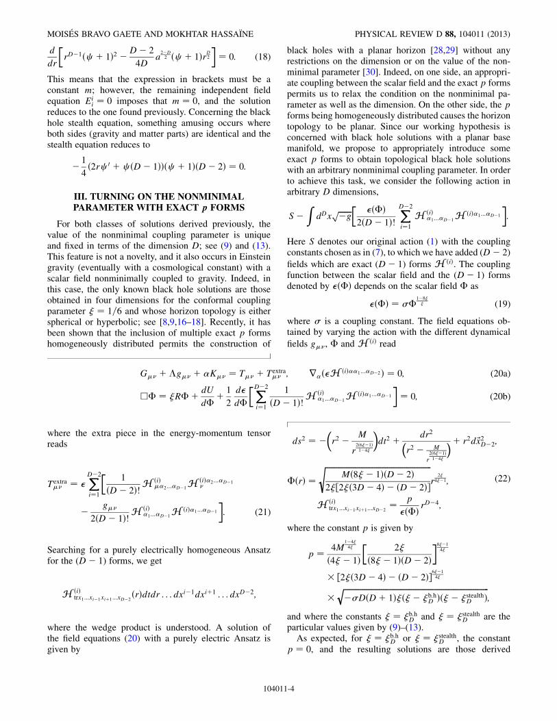
d
dr
rD1ðc þ 1Þ2 D 2
4Da
2D2 ðc þ 1ÞrD2
¼ 0: (18)
This means that the expression in brackets must be aconstant m; however, the remaining independent fieldequation Ei
i ¼ 0 imposes that m ¼ 0, and the solutionreduces to the one found previously. Concerning the blackhole stealth equation, something amusing occurs whereboth sides (gravity and matter parts) are identical and thestealth equation reduces to
1
4ð2rc 0 þ c ðD 1ÞÞðc þ 1ÞðD 2Þ ¼ 0:
III. TURNING ON THE NONMINIMALPARAMETER WITH EXACT p FORMS
For both classes of solutions derived previously, thevalue of the nonminimal coupling parameter is uniqueand fixed in terms of the dimension D; see (9) and (13).This feature is not a novelty, and it also occurs in Einsteingravity (eventually with a cosmological constant) with ascalar field nonminimally coupled to gravity. Indeed, inthis case, the only known black hole solutions are thoseobtained in four dimensions for the conformal couplingparameter ¼ 1=6 and whose horizon topology is eitherspherical or hyperbolic; see [8,9,16–18]. Recently, it hasbeen shown that the inclusion of multiple exact p formshomogeneously distributed permits the construction of
black holes with a planar horizon [28,29] without anyrestrictions on the dimension or on the value of the non-minimal parameter [30]. Indeed, on one side, an appropri-ate coupling between the scalar field and the exact p formspermits us to relax the condition on the nonminimal pa-rameter as well as the dimension. On the other side, the pforms being homogeneously distributed causes the horizontopology to be planar. Since our working hypothesis isconcerned with black hole solutions with a planar basemanifold, we propose to appropriately introduce someexact p forms to obtain topological black hole solutionswith an arbitrary nonminimal coupling parameter. In orderto achieve this task, we consider the following action inarbitrary D dimensions,
SZ
dDxffiffiffiffiffiffiffig
p ðÞ
2ðD 1Þ!XD2
i¼1
H ðiÞ1...D1
H ðiÞ1...D1
:
Here S denotes our original action (1) with the couplingconstants chosen as in (7), to which we have added (D 2)
fields which are exact (D 1) forms H ðiÞ. The couplingfunction between the scalar field and the (D 1) formsdenoted by ðÞ depends on the scalar field as
ðÞ ¼ 18 (19)
where is a coupling constant. The field equations ob-tained by varying the action with the different dynamical
fields g, and H ðiÞ read
G þg þ K ¼ T þ Textra ; rðH ðiÞ1...D2Þ ¼ 0; (20a)
h ¼ Rþ dU
dþ 1
2
d
d
XD2
i¼1
1
ðD 1Þ!HðiÞ1...D1
H ðiÞ1...D1
¼ 0; (20b)
where the extra piece in the energy-momentum tensorreads
Textra ¼
XD2
i¼1
1
ðD 2Þ!HðiÞ2...D1
H ðiÞ2...D1
g
2ðD 1Þ!HðiÞ1...D1
H ðiÞ1...D1
: (21)
Searching for a purely electrically homogeneous Ansatzfor the (D 1) forms, we get
H ðiÞtrx1...xi1xiþ1...xD2
ðrÞdtdr . . . dxi1dxiþ1 . . .dxD2;
where the wedge product is understood. A solution ofthe field equations (20) with a purely electric Ansatz isgiven by
ds2 ¼ r2 M
r2ð61Þ14
dt2 þ dr2
r2 M
r2ð61Þ14
þ r2d~x2D2;
ðrÞ ¼ffiffiffiffiffiffiffiffiffiffiffiffiffiffiffiffiffiffiffiffiffiffiffiffiffiffiffiffiffiffiffiffiffiffiffiffiffiffiffiffiffiffiffiffiffiffiffiffiffiffiffiffiffiffiffiffi
Mð8 1ÞðD 2Þ2½2ð3D 4Þ ðD 2Þ
sr
241;
H ðiÞtrx1...xi1xiþ1...xD2
¼ p
ðÞ rD4;
(22)
where the constant p is given by
p ¼ 4M144
ð4 1Þ
2
ð8 1ÞðD 2Þ81
4
½2ð3D 4Þ ðD 2Þ614
ffiffiffiffiffiffiffiffiffiffiffiffiffiffiffiffiffiffiffiffiffiffiffiffiffiffiffiffiffiffiffiffiffiffiffiffiffiffiffiffiffiffiffiffiffiffiffiffiffiffiffiffiffiffiffiffiffiffiffiffiffiffiffiffiffiffiffiffiffiffiffiffiffiffiffiffiffiDðDþ 1Þð b:h
D Þð stealthD Þ
q;
and where the constants ¼ b:hD and ¼ stealth
D are theparticular values given by (9)–(13).As expected, for ¼ b:h
D or ¼ stealthD , the constant
p ¼ 0, and the resulting solutions are those derived
MOISES BRAVO GAETE AND MOKHTAR HASSAINE PHYSICAL REVIEW D 88, 104011 (2013)
104011-4
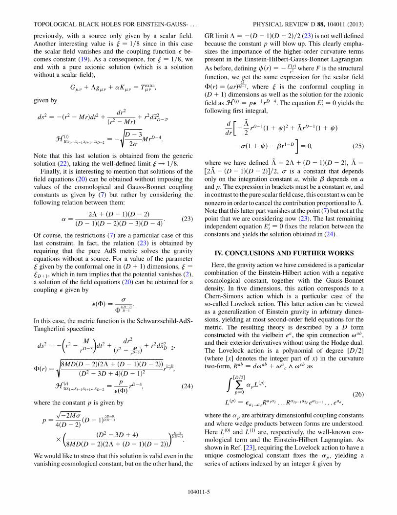
previously, with a source only given by a scalar field.Another interesting value is ¼ 1=8 since in this casethe scalar field vanishes and the coupling function be-comes constant (19). As a consequence, for ¼ 1=8, weend with a pure axionic solution (which is a solutionwithout a scalar field),
G þg þ K ¼ Textra ;
given by
ds2 ¼ ðr2 MrÞdt2 þ dr2
ðr2 MrÞ þ r2d~x2D2;
H ðiÞtrx1...xi1xiþ1...xD2
¼ ffiffiffiffiffiffiffiffiffiffiffiffiffiD 3
2
sMrD4:
Note that this last solution is obtained from the genericsolution (22), taking the well-defined limit ! 1=8.
Finally, it is interesting to mention that solutions of thefield equations (20) can be obtained without imposing thevalues of the cosmological and Gauss-Bonnet couplingconstants as given by (7) but rather by considering thefollowing relation between them:
¼ 2þ ðD 1ÞðD 2ÞðD 1ÞðD 2ÞðD 3ÞðD 4Þ : (23)
Of course, the restrictions (7) are a particular case of thislast constraint. In fact, the relation (23) is obtained byrequiring that the pure AdS metric solves the gravityequations without a source. For a value of the parameter given by the conformal one in (Dþ 1) dimensions, ¼Dþ1, which in turn implies that the potential vanishes (2),a solution of the field equations (20) can be obtained for acoupling given by
ðÞ ¼
4ðD2ÞD1
:
In this case, the metric function is the Schwarzschild-AdS-Tangherlini spacetime
ds2 ¼ r2 M
rD3
dt2 þ dr2
ðr2 MrD3Þ þ r2d~x2D2;
ðrÞ ¼ffiffiffiffiffiffiffiffiffiffiffiffiffiffiffiffiffiffiffiffiffiffiffiffiffiffiffiffiffiffiffiffiffiffiffiffiffiffiffiffiffiffiffiffiffiffiffiffiffiffiffiffiffiffiffiffiffiffiffiffiffiffiffiffiffiffiffiffiffiffiffiffiffiffiffiffi8MDðD 2Þð2þ ðD 1ÞðD 2ÞÞ
ðD2 3Dþ 4ÞðD 1Þ2s
r1D2 ;
H ðiÞtrx1...xi1xiþ1...xD2
¼ p
ðÞ rD4; (24)
where the constant p is given by
p ¼ffiffiffiffiffiffiffiffiffiffiffiffiffiffiffi2M
p4ðD 2Þ ðD 1Þ 5D9
2ðD1Þ
ðD2 3Dþ 4Þ8MDðD 2Þð2þ ðD 1ÞðD 2ÞÞ
D32ðD1Þ
:
Wewould like to stress that this solution is valid even in thevanishing cosmological constant, but on the other hand, the
GR limit ¼ ðD 1ÞðD 2Þ=2 (23) is not well definedbecause the constant p will blow up. This clearly empha-sizes the importance of the higher-order curvature termspresent in the Einstein-Hilbert-Gauss-Bonnet Lagrangian.
As before, defining c ðrÞ ¼ FðrÞr2
where F is the structural
function, we get the same expression for the scalar field
ðrÞ ¼ ðarÞ 241, where is the conformal coupling in
(Dþ 1) dimensions as well as the solution for the axionic
field asH ðiÞ ¼ p1rD4. The equation Ett ¼ 0 yields the
following first integral,
d
dr
~
2rD1ð1þ c Þ2 þ rD1ð1þ c Þ
ð1þ c Þ r1D
¼ 0; (25)
where we have defined ~ ¼ 2þ ðD 1ÞðD 2Þ, ¼½2~ ðD 1ÞðD 2Þ=2, is a constant that dependsonly on the integration constant a, while depends on aand p. The expression in brackets must be a constantm, andin contrast to the pure scalar field case, this constantm can be
nonzero in order to cancel the contribution proportional to .Note that this latter part vanishes at the point (7) but not at thepoint that we are considering now (23). The last remainingindependent equation Ei
i ¼ 0 fixes the relation between theconstants and yields the solution obtained in (24).
IV. CONCLUSIONS AND FURTHER WORKS
Here, the gravity action we have considered is a particularcombination of the Einstein-Hilbert action with a negativecosmological constant, together with the Gauss-Bonnetdensity. In five dimensions, this action corresponds to aChern-Simons action which is a particular case of theso-called Lovelock action. This latter action can be viewedas a generalization of Einstein gravity in arbitrary dimen-sions, yielding at most second-order field equations for themetric. The resulting theory is described by a D formconstructed with the vielbein ea, the spin connection !ab,and their exterior derivatives without using the Hodge dual.The Lovelock action is a polynomial of degree [D=2](where [x] denotes the integer part of x) in the curvaturetwo-form, Rab ¼ d!ab þ!a
c ^!cb as
Z X½D=2
p¼0
pLðpÞ;
LðpÞ ¼ a1...adRa1a2 . . .Ra2p1a2pea2pþ1 . . . ead ;
(26)
where thep are arbitrary dimensionful coupling constants
and where wedge products between forms are understood.
Here Lð0Þ and Lð1Þ are, respectively, the well-known cos-mological term and the Einstein-Hilbert Lagrangian. Asshown in Ref. [23], requiring the Lovelock action to have aunique cosmological constant fixes the p, yielding a
series of actions indexed by an integer k given by
TOPOLOGICAL BLACK HOLES FOR EINSTEIN-GAUSS- . . . PHYSICAL REVIEW D 88, 104011 (2013)
104011-5

Ik ¼Z Xk
p¼0
Ckp
ðD2pÞLðpÞ; 1 k
D1
2
; (27)
where Ckp corresponds to the combinatorial factors. The
gravity action we have considered here (8) is nothing butthe action I2 given by the expression (27). We believe thatthe class of solutions derived here for I2 can be generalizedfor an arbitrary gravity action Ik with k 2 [21]. Forexample, the stealth black hole solution obtained for I2can easily be extended for an arbitrary action Ik by adjust-ing the value of the nonminimal coupling parameter ap-pearing in the stealth metric solution (17) in order for theresulting metric to match with the pure gravity solution ofIk [23,24]. Moreover, to our knowledge, there do not existblack hole solutions with a planar base manifold for stan-dard general relativity (with or without a cosmologicalconstant) with a source given by a nonminimally coupledscalar field [31]. This reinforces our conviction that theexistence of the solutions derived for a gravity action givenby I2 is strongly indicative of the presence of the higher-order curvature terms [21].
We now turn to the choice of the mass term potential (2)in our starting action. First of all, we may note that thiskind of potential has been considered in the dual descrip-tion of unconventional superconductor [2,4–6]. Moreover,in our case, because of the presence of the nonminimalcoupling term R2 in the action, in the case of constantscalar curvature solutions R ¼ DðD 1Þ, one may de-fine an effective square mass
m2eff ¼DðD1Þ
1 16
ð14Þ2 ðDÞðDþ1Þ:
In the solutions obtained here, the only ones of constantscalar curvature (apart from the trivial situation of takingM ¼ 0) are those with the p-form fields (22) for ¼D=ð4Dþ 4Þ and ¼ ðD 1Þ=ð4DÞ. It is interesting tonote that the square effective mass m2
eff precisely saturates
the Breitenlohner-Freedman bound for ¼ ðD 1Þ=ð4DÞ.To close the chapter concerning the potential, we stress thatis a particular case of potentials allowing the existence of aself-interacting scalar field nonminimally coupled to thevanishing stress tensor
T :¼ @@ g
1
2@@þUðÞ
þ ðghrr þGÞ2 ¼ 0
on the AdS background
ds2 ¼ r2dt2 þ dr2
r2þ r2d~x2D2:
Indeed, as shown in [22], the stealth solution is given by thefollowing configuration,
UðÞ ¼
ð1 4Þ2 ½2b2
12 8ðD 1Þð DÞ
ð2b12 Dð Dþ1Þ2Þ; (28a)
ðrÞ ¼ ðArþ bÞ 241: (28b)
Note that this kind of potential also appears when lookingfor AdS wave solutions for a nonminimally coupledscalar field [32]. The scalar field solutions obtained inthis paper, as well as the potential considered, correspondto the b ¼ 0 limit of this stealth configuration (28). It hasbeen shown recently that, in the context of standardgeneral relativity, self-interacting scalar fields nonmini-mally coupled with the potential given by (28a) and extraaxionic fields admit black hole solutions [30]. The deri-vation of these solutions was precisely operated fromthe stealth configuration (28) through a Kerr-Schildtransformation [30]. We believe that there may existmore general black hole solutions than those derivedhere for this more general class of potentials (28a). Toconclude with the stealth origin, we would like to stressthat the horizon topology of our solutions is planar, andtheir extension to spherical or hyperboloid black holesolutions in a standard fashion is not possible. This maybe related to the fact that a static stealth scalar field on theAdS background requires the base space to be flat [22]for dimensions D 4.An interesting task to realize will be the study of the
thermodynamics properties of the solutions derived herefor I2 as well as those for general Ik, and to compare themwith the pure gravity solutions [24].In Ref. [33], the authors constructed a conformal cou-
pling to arbitrary higher-order Euler densities. It will beinteresting to see whether such a matter source can accom-modate the kind of solutions derived here.As a final remark, we note that the coupling with the
Maxwell electromagnetic field is an open problem even inthe black hole stealth case. Indeed, even if the pure gravitysolution with the Maxwell source
G þg þ K ¼ TMaxwell
is known [23,24], it seems that this solution cannot bepromoted to a black hole stealth configuration with anonminimal scalar field as was possible in the neutralcase.
ACKNOWLEDGMENTS
We thank Julio Oliva and Sourya Ray for useful discus-sions. M. B. is supported by BECA DOCTORALCONICYT 21120271. M.H. was partially supported byGrant No. 1130423 from FONDECYT, by Grant No. ACT56 from CONICYT, and by CONICYT, Departamento deRelaciones Internacionales ‘‘Programa RegionalMATHAMSUD 13 MATH-05.’’ We thank the referee forits instructive comments.
MOISES BRAVO GAETE AND MOKHTAR HASSAINE PHYSICAL REVIEW D 88, 104011 (2013)
104011-6

[1] J.M. Maldacena, Adv. Theor. Math. Phys. 2, 231(1998).
[2] S. A. Hartnoll, Classical Quantum Gravity 26, 224002(2009).
[3] Y. V. Kovchegov, Rep. Prog. Phys. 75, 124301 (2012).[4] G. T. Horowitz, arXiv:1002.1722.[5] S. A. Hartnoll, C. P. Herzog, and G. T. Horowitz, J. High
Energy Phys. 12 (2008) 015.[6] C. P. Herzog, J. Phys. A 42, 343001 (2009).[7] J. D. Bekenstein, arXiv:gr-qc/9808028.[8] J. D. Bekenstein, Ann. Phys. (Berlin) 82, 535 (1974).[9] N.M. Bocharova, K.A. Bronnikov, and V.N. Melnikov,
Vestn. Mosk. Univ. Fiz. Astron. 6, 706 (1970) [MoscowUniv. Phys. Bull. 25, 80 (1970)].
[10] L. Barclay, R. Gregory, S. Kanno, and P. Sutcliffe, J. HighEnergy Phys. 12 (2010) 029.
[11] W. Yao and J. Jing, J. High Energy Phys. 05 (2013)101.
[12] S.-l. Cui and Z. Xue, arXiv:1306.2013.[13] C. Charmousis, Lect. Notes Phys. 769, 299 (2009).[14] C. Garraffo and G. Giribet, Mod. Phys. Lett. A 23, 1801
(2008).[15] J. P. S. Lemos, Classical Quantum Gravity 12, 1081
(1995); Phys. Lett. B 353, 46 (1995).[16] C. Martinez, R. Troncoso, and J. Zanelli, Phys. Rev. D 67,
024008 (2003).[17] C. Martinez, J. P. Staforelli, and R. Troncoso, Phys. Rev. D
74, 044028 (2006).[18] A. Anabalon and A. Cisterna, Phys. Rev. D 85, 084035
(2012).
[19] E. Ayon-Beato, C. Martinez, and J. Zanelli, Gen. Relativ.Gravit. 38, 145 (2006).
[20] M. Banados, C. Teitelboim, and J. Zanelli, Phys. Rev. Lett.69, 1849 (1992).
[21] M. Bravo-Gaete and M. Hassaine (work in progress).[22] E. Ayon-Beato, C. Martinez, R. Troncoso, and J. Zanelli
(private communication).[23] J. Crisostomo, R. Troncoso, and J. Zanelli, Phys. Rev. D
62, 084013 (2000).[24] R. Aros, R. Troncoso, and J. Zanelli, Phys. Rev. D 63,
084015 (2001).[25] Note that solutions of the Einstein-Gauss-Bonnet equa-
tions with arbitrary coupling constants were first obtainedin the case ¼ 0 with a spherical topology in [26] and anarbitrary topology in [27].
[26] D. G. Boulware and S. Deser, Phys. Rev. Lett. 55, 2656(1985).
[27] R.-G. Cai, Phys. Rev. D 65, 084014 (2002).[28] Y. Bardoux, M.M. Caldarelli, and C. Charmousis, J. High
Energy Phys. 05 (2012) 054.[29] Y. Bardoux, M.M. Caldarelli, and C. Charmousis,
arXiv:1205.4025.[30] M.M. Caldarelli, C. Charmousis, and M. Hassaine, J.
High Energy Phys. 10 (2013) 015.[31] There exist solutions adding exact p forms coupled to the
scalar field; see [29,30].[32] E. Ayon-Beato and M. Hassaine, Phys. Rev. D 73, 104001
(2006).[33] J. Oliva and S. Ray, Classical Quantum Gravity 29,
205008 (2012).
TOPOLOGICAL BLACK HOLES FOR EINSTEIN-GAUSS- . . . PHYSICAL REVIEW D 88, 104011 (2013)
104011-7

JHEP11(2013)177
Published for SISSA by Springer
Received: September 23, 2013
Revised: October 31, 2013
Accepted: November 15, 2013
Published: November 25, 2013
Planar AdS black holes in Lovelock gravity with a
nonminimal scalar field
Moises Bravo Gaete and Mokhtar Hassaıne
Instituto de Matematica y Fısica, Universidad de Talca,
Casilla 747, Talca, Chile
E-mail: mbravog-at-inst-mat.utalca.cl, hassaine-at-inst-mat.utalca.cl
Abstract: In arbitrary dimension D, we consider a self-interacting scalar field nonmini-
mally coupled with a gravity theory given by a particular Lovelock action indexed by an
integer k. To be more precise, the coefficients appearing in the Lovelock expansion are fixed
by requiring the theory to have a unique AdS vacuum with a fixed value of the cosmo-
logical constant. This yields to k = 1, 2, · · · ,[D−12
]inequivalent possible gravity theories;
here the case k = 1 corresponds to the standard Einstein-Hilbert Lagrangian. For each
par (D, k), we derive two classes of AdS black hole solutions with planar event horizon
topology for particular values of the nonminimal coupling parameter. The first family of
solutions depends on a unique constant and is valid only for k ≥ 2. In fact, its GR coun-
terpart k = 1 reduces to the pure AdS metric with a vanishing scalar field. The second
family of solutions involves two independent constants and corresponds to a stealth black
hole configuration; that is a nontrivial scalar field together with a black hole metric such
that both side of the Einstein equations (gravity and matter parts) vanishes identically.
In this case, the standard GR case k = 1 reduces to the Schwarzschild-AdS-Tangherlini
black hole metric with a trivial scalar field. We show that the two-parametric stealth solu-
tion defined in D dimension can be promoted to the uniparametric black hole solution in
(D+1) dimension by fixing one of the two constants in term of the other and by adding a
transversal coordinate. In both cases, the existence of these solutions is strongly inherent
of the presence of the higher order curvature terms k ≥ 2 of the Lovelock gravity. We
also establish that these solutions emerge from a stealth configuration defined on the pure
AdS metric through a Kerr-Schild transformation. Finally, in the last part, we include
multiple exact (D − 1)−forms homogenously distributed and coupled to the scalar field.
For a specific coupling, we obtain black hole solutions for arbitrary value of the nonminimal
coupling parameter generalizing those obtained in the pure scalar field case.
Keywords: Classical Theories of Gravity, Black Holes
ArXiv ePrint: 1309.3338
c© SISSA 2013 doi:10.1007/JHEP11(2013)177

JHEP11(2013)177
Contents
1 Introduction 1
2 Planar AdS black holes for a particular Lovelock gravity with a nonmin-
imal scalar field 3
2.1 Planar AdS black hole solutions 5
2.2 Planar AdS black hole stealth solutions 6
3 Adding exact (D − 1)-forms 8
4 Comments and conclusions 10
A Complements concerning the solutions 12
A.1 Stealth origin of the solutions 12
A.2 Particular case of Einstein gravity k = 1 14
1 Introduction
Since the advent of string theory, the interests on higher-dimensional physics have grown
up in the last decades, and particulary concerning the higher-dimensional General Rela-
tivity (GR). String corrections to the standard higher-dimensional Einstein-Hilbert action
arise as a low energy expansion in powers in α′ and involve higher powers of the curva-
tures. As shown in [1] and [2], in order to the graviton amplitude to be ghost-free a special
combination of quadratic corrections which is nothing but the Gauss-Bonnet expression is
required. One of the interesting features of the Gauss-Bonnet Lagrangian lies in the fact
that its variation yields second-order field equations for the metric in spite of the presence of
quadratic terms in the curvature. The Einstein-Hilbert-Gauss-Bonnet gravity piece is part
of a more general gravity theory build out of the same principles as GR. Indeed, two of the
main fundamental assumptions in GR are the requirements of general covariance and the
fact that the field equations for the metric to be at most of second order. In view of this, it
is natural to describe the spacetime geometry in three or four dimensions by the standard
Einstein-Hilbert action (with eventually a cosmological constant term) while for dimensions
greater than four a more general theory can be used. This fact has been first noticed by
Lanczos in five dimensions [3] and then generalized in higher dimension D by Lovelock [4].
The resulting action is the so-called Lovelock gravity action which is a D−form constructed
out of the vielbein, the spin connection and their exterior derivative. By construction, the
Lovelock Lagrangian which contains higher powers of the curvatures remains invariant un-
der local Lorentz transformations. In odd dimension, this gauge symmetry can be extended
to a local anti de Sitter (AdS) or Poincare symmetry through a particular choice of the
– 1 –

JHEP11(2013)177
coefficients appearing in the Lovelock expansion. In both cases, the resulting Lagrangian is
a Chern-Simons form since its exterior derivative is an invariant homogeneous polynomial
in the AdS or Poincare curvatures, and their supersymmetric extensions are also known;
see [5] for a good review on Chern-Simons (super)gravity. The Lovelock gravity or its
Chern-Simons particular case have been shown to possess (topological) AdS black hole
solutions with interesting thermodynamical properties [6–9] generalizing those obtained in
the Einstein-Gauss-Bonnet case [10, 11]; for good reviews on Einstein-Gauss-Bonnet black
holes, see e.g. [12–14].
In the present work, we will consider a gravity action given by a particular Lovelock
Lagrangian with fixed coefficients such that the resulting theory has a unique anti-de Sitter
vacuum with a fixed cosmological constant while our matter action will be concerned with
a nonminimal self-interacting scalar field. For this Lovelock gravity model with nonmini-
mal scalar field source, we will look for topological black hole solutions with planar event
horizon topology. Note that the first examples of topological black holes in GR without
source were discussed in [15, 16]. The reasons of considering such a matter source are mul-
tiples. Firstly, the ideas behind the anti-de Sitter/Conformal Field Theory (AdS/CFT)
correspondence [17] have been recently extended to non-relativistic physics particularly to
gain a better understanding of some unconventional superconductors [18–20]. In this con-
text, black holes with scalar hair at low temperature which disappears at low temperature
play an important role since they will reproduce the correct behavior of the superconductor
phase diagram. It is well-known now from the BBMB solution (solution of the Einstein
equations with a conformal source given by a scalar field) in four dimensions [21, 22] that
scalar fields nonminimally coupled can be useful to escape standard no-hair theorems [23].
Note that the BBMB solution has been extended in presence of a cosmological constant
with a potential term in four dimensions and for the conformal nonminimal coupling pa-
rameter ξ = 1/6, [24–27]. In fact, scalar fields nonminimally coupled to curved spacetimes
play an important role in different branches of physics and are also of interest for pure
mathematical proposals (as for example for the Yamabe problem). The introduction of
nonminimal couplings in spite of complicating the calculations may be of extreme rele-
vance for many problems. For example, the nonminimal couplings are generated by quan-
tum corrections even if they are absent in the classical action [28], and they are required
in order to renormalize the theory or at least to enhance their renormalizability proper-
ties [29–31]. In cosmological context, it has been argued that in most of the inflationary
scenarios with scalar fields, the presence of the nonminimal coupling is unavoidable and its
correct value depends on the gravity and the scalar field models adopted [32, 33]. Secondly,
we have already considered such matter source in the case of a particular combination of
the Einstein-Hilbert-Gauss-Bonnet gravity action and establish the existence of some black
hole configurations for particular values of the nonminimal coupling parameter [34]. The
present work is then the natural extension of the work done in [34] in order to reinforce
our conviction that these black hole solutions are strongly inherent to the presence of the
higher-order curvature terms.
The plan of the paper is organized as follows. In the next section, we present the
model of a scalar field nonminimally coupled with a gravity action given by a particular
– 2 –
JHEP11(2013)177
Lovelock Lagrangian. After deriving the field equations, we will present two classes of
topological black hole solutions with planar base manifold. In section 3, we will add to the
starting action exact (D−1)−forms and obtain a more general class of black hole solutions
generalizing those obtained in the pure scalar field case. Finally, the last section is devoted
to our conclusions, comments and further works. Two appendices are also added. In
the first one, we show that these black hole solutions can be constructed from a stealth
configuration on the pure AdS metric through a Kerr-Schild transformation. In the second
appendix, we establish that the existence of these solutions is inherent to the higher-order
curvature terms k ≥ 2 of the Lovelock Lagrangian and they can not be promoted to black
hole solutions in the standard GR case k = 1.
2 Planar AdS black holes for a particular Lovelock gravity with a non-
minimal scalar field
We start with a generalization of the Einstein-Hilbert gravity action in arbitrary dimension
D yielding at most to second-order field equations for the metric and known as the Lovelock
Lagrangian. This latter is a D−form constructed with the vielbein ea, the spin connection
ωab, and their exterior derivatives without using the Hodge dual. The Lovelock action is
a polynomial of degree [D/2] (where [x] denotes the integer part of x) in the curvature
two-form, Rab = dωab + ωac ∧ ωcb as
∫ [D/2]∑
p=0
αp L(p), (2.1a)
L(p) = ǫa1···adRa1a2 · · ·Ra2p−1a2pea2p+1 · · · ead , (2.1b)
where the αp are arbitrary dimensionful coupling constants and where wedge products
between forms are understood. Here L(0) and L(1) are proportional respectively to the
cosmological term and the Einstein-Hilbert Lagrangian. Now, as shown in ref. [8], requiring
the Lovelock action to have a unique AdS vacuum with a unique cosmological constant,
fixes the αp yielding to a series of actions indexed by an integer k, and given by
Ik = − 1
2k(D − 3)!
∫ k∑
p=0
Ckp
(D − 2p)L(p), 1 ≤ k ≤
[D − 1
2
], (2.2)
where Ckp corresponds to the combinatorial factor. The global factor in front of the integral
is chosen such that the gravity action (2.2) can be re-written in the standard fashion as
Ik =1
2
∫dDx
√−g
[R+
(D − 1)(D − 2)
k+
(k − 1)
2(D − 3)(D − 4)LGB +
(k − 1)(k − 2)
3!(D − 3)(D − 4)(D − 5)(D − 6)L(3) + · · ·
], (2.3)
– 3 –
JHEP11(2013)177
where LGB = R2 − 4RµνRµν +RαβµνR
αβµν stands for the Gauss-Bonnet Lagrangian, and
L(3) is given by
L(3) = R3 − 12RRµνRµν + 16RµνR
µρR
νρ + 24RµνRρσRµρνσ + 3RRµνρσR
µνρσ
−24RµνRµρσκR
νρσκ + 4RµνρσRµνηζRρσ
ηζ − 8RµρνσRµ νη ζR
ρησζ .
Note that in odd dimension D = 2n−1 and for k = n−1, the corresponding action In−1 is
a Chern-Simons action, that is a (2n−1)−form whose exterior derivative can be written as
the contraction of an invariant tensor with the wedge product of n curvatures two-forms.
In even dimension D = 2n, the maximal value of k is n− 1, and in this case the resulting
gravity action has a Born-Infeld like structure since it can be written as the Pfaffian of
the 2−form Rab = Rab + eaeb. The gravity theories Ik have been shown to possess black
hole solutions with interesting features, in particular concerning their thermodynamics
properties, see [8] and [9]. In what follows, we will consider a scalar field nonminimally
coupled together with the gravity actions given by Ik, (2.2). More precisely, we will consider
the following action for any integer k ≥ 2,1
Sk =Ik −∫
dDx√−g
[1
2∂µΦ∂
µΦ+ξ
2RΦ2 + U(Φ)
], (2.4)
The field equations read
G(k)µν = Tµν , (2.5a)
Φ = ξRΦ+dU
dΦ, (2.5b)
where G(k)µν is the gravity tensor associated to the variation of the action Ik (2.2),
G(k)µν = Gµν −
(D − 1)(D − 2)
2kgµν +
(k − 1)
2(D − 3)(D − 4)Kµν +
(k − 1)(k − 2)
3!(D − 3)(D − 4)(D − 5)(D − 6)Sµν + · · ·
where Kµν is the Gauss-Bonnet tensor
Kµν = 2(RRµν − 2RµρR
ρν − 2RρσRµρνσ +R ρσγ
µ Rνρσγ
)− 1
2gµνLGB
and Sµν arises from the variation of L(3),
Sµν = 3(R2Rµν − 4RRρµR
ρν − 4RρσRρσRµν + 8RρσRρµRσν − 4RRρσRρµσν
+8RρκRσκRρµσν − 16RρσRκ
(µR|κσρ|ν) + 2RRρσκµRρσκν +RµνR
ρσκηRρσκη
−8Rρ(µR
σκη|ρ|R|σκη|ν) − 4RρσRκη
ρµRκησν + 8RρσRρκσηRκµην − 8RρσR
ρκηµR
σκην
+4RρσκηRρσζµRζ
κη ν − 8RρκσηRζρσµRζκην − 4Rρσκ
ηRρσκζRη ζµ ν
)− 1
2gµνL(3).
1The standard GR case k = 1 will be discussed in the appendix.
– 4 –

JHEP11(2013)177
In the matter part of the equations (2.5), Tµν represents the energy-momentum tensor of
the scalar field given by
Tµν = ∂µΦ∂νΦ− gµν
(1
2∂σΦ∂
σΦ+ U(Φ)
)+ ξ (gµν−∇µ∇ν +Gµν) Φ
2, (2.6)
where the potential U(Φ) is given by a mass term
U(Φ) =8 ξ D (D − 1)
(1− 4ξ)2(ξ − ξD)(ξ − ξD+1)Φ
2, (2.7)
where ξD denotes the conformal coupling in D dimensions
ξD =D − 2
4(D − 1). (2.8)
The choice of such potential will be justified in the appendix. Being a mass term and
because of the presence of the term ξRΦ2 in the action, one can define an effective mass
m2eff in the case of solutions of constant curvature R = constant by
m2eff = ξR+
16 ξ D (D − 1)
(1− 4ξ)2(ξ − ξD)(ξ − ξD+1). (2.9)
As for the Einstein-Gauss-Bonnet case k = 2 [34], we will obtain the same two classes
of black hole solutions for generic value of k ≥ 2. More precisely, for each par (D, k) with
D ≥ 5 and k ≥ 2 , we will derive two classes of AdS black hole solutions with planar event
horizon topology for specific values of the nonminimal coupling parameter ξ.
2.1 Planar AdS black hole solutions
For k ≥ 2, an AdS black hole solution is obtained provided that the nonminimal parameter
ξ takes the following form
ξb.hk,D =
(D − 2)(k − 1)
4[(D − 1)k − (D − 2)
] , (2.10)
which in turn implies that the potential (2.7) becomes
Ub.hk,D(Φ) =
(k − 1)(D − 2)2(D − 2 + k)
8k2[(D − 1)k − (D − 2)
] Φ2. (2.11)
In this case, the metric solution and the scalar field are given by
ds2 = −F b.hk,D(r)dt
2 +dr2
F b.hk,D(r)
+ r2d~x2D−2,
F b.hk,D(r) = r2 − M
rD−2(k+1)
k
, (2.12)
Φb.hk,D(r) = M
k−12
√4 [(D − 1)k − (D − 2)]
(k − 1)(D − 2)r
(k−1)(2−D)2k .
– 5 –

JHEP11(2013)177
Many comments can be made concerning this solution. Firstly, this black hole solution
depends on a unique integration constant M , and for even k the scalar field is always real
provided that M is positive constant while for odd k, the constant M can be positive or
negative. The scalar field is well defined at the horizon and blows-up at the singularity
r = 0. The solution given by (2.10), (2.11), (2.12) reduces to the one derived in the
Einstein-Gauss-Bonnet case for k = 2 [34]. It is interesting to note that the standard
GR-limit k = 1 (which yields to Einstein gravity with a negative cosmological constant) is
possible only in the limit M = 0 as it can be seen from the expression of the scalar field.
This is not surprising since for k = 1, the nonminimal coupling parameter (2.10) as well as
the potential (2.11) vanish, and in this case, no-hair theorems forbid the existence of black
hole solutions. We will come in detail to this point in the appendix. We would like also
to emphasize that the allowed value of the nonminimal coupling parameter (2.10) which
depends on (k,D) is bounded as ξb.hk,D < 1/4 and its limit as k goes to infinity yields to
the conformal coupling in D dimensions, limk→∞ ξb.hk,D = ξD. Finally, we may observe that
in even dimension given by D = 2(k + 1) which corresponds to the Born-Infeld case, the
lapse function F b.hk,D(r) has a BTZ-like form [35] as it occurs in the vacuum case with a base
manifold chosen to be non-Einstein [36].
2.2 Planar AdS black hole stealth solutions
The black hole stealth solution for k ≥ 2 can be obtained in analogue way that the one
obtained in the Einstein-Gauss-Bonnet case k = 2 [34]; this means by combining the pure
gravity solution with planar base manifold [8, 9] with the stealth configuration. By stealth
configuration, we mean a non-trivial solution (with a non constant scalar field) of the
stealth equations
G(k)µν = 0 = Tµν , (2.13)
where both side (gravity and matter part) vanishes.
In fact, it is not difficult to show that a self-interacting nonminimal scalar field given by
Φ(r) = Ar2ξ
4ξ−1 , (2.14)
has a vanishing energy-momentum tensor (2.6) Tµν = 0 on the following ξ−dependent
spacetime geometry
ds2 = −(r2 − M
r4(D−2)ξ−(D−3)
4ξ−1
)dt2 +
dr2(r2 − M
r4(D−2)ξ−(D−3)
4ξ−1
) + r2d~x2D−2. (2.15)
On the other hand, the pure gravity equations G(k)µν = 0 has a black hole solution with a
lapse function F (r) given by [8, 9]
F (r) = r2 − M
rD−(2k+1)
k
.
– 6 –
JHEP11(2013)177
Now, in order for this metric function to coincide with the stealth metric (2.15), the non-
minimal coupling parameter must be chosen as
ξstealthk,D =
(D − 1)(k − 1)
4 [Dk − (D − 1)], (2.16)
and hence the mass term potential (2.7) becomes
U stealthk,D (Φ) =
(k − 1)(D − 1)2(D − 1− k)
8k2 [Dk − (D − 1)]Φ2. (2.17)
Consequently, a topological black hole stealth solution of the stealth equation (2.13) is
given by
ds2 = −F stealthk,D (r)dt2 +
dr2
F stealthk,D (r)
+ r2d~x2D−2,
F stealthk,D (r) = r2 − M
rD−(2k+1)
k
, (2.18)
Φstealthk,D (r) = Ar
(k−1)(1−D)2k .
We may note that in contrast with the previous solution, the black hole stealth solution
depends on two integration constants M and A, and in the vanishing M limit, the solution
reduces to a stealth solution on the pure AdS background [37]. The GR limit k = 1 is
also well defined yielding to a metric that is noting but the topological Schwarzschild-
AdS-Tangherlini spacetime. This is not surprising since in the GR limit case k = 1,
the nonminimal coupling parameter as well as the potential vanish while the scalar field
becomes constant, and hence the energy-momentum tensor vanishes Tµν = 0. In other
words, in the GR-limit, the stealth equations (2.13) are equivalent to the pure Einstein
equations Gµν − (D−1)(D−2)2 gµν = 0. This class of solutions is of particular interest since,
up to now, the only black hole stealth solution was the one obtained in [38] in the three-
dimensional GR case with a static BTZ metric [35].
Let us go back to the ξ−dependent geometry (2.15) allowing the existence of solution
of Tµν = 0. It is clear from the expression of the metric that for a nonminimal coupling
parameter ξ ∈ [ξD+1,14 [ where ξD+1 = (D − 1)/(4D) is the conformal coupling in (D + 1)
dimension, the asymptotic behavior of the metric as r → ∞ is faster than the usual AdS
one. However, requiring the metric to be also solution of the gravity part G(k)µν = 0, we
have seen that the parameter ξ must take the form (2.16), and it is not difficult to prove
that ξstealthk,D < ξD+1. To conclude, we would like to point out a certain symmetry between
the black hole and stealth solution as reflected by the following relations
ξstealthk,D = ξb.h
k,D+1, F stealthk,D = F b.h
k,D+1, U stealthk,D = Ub.h
k,D+1, Φstealthk,D ∝ Φb.h
k,D+1.
These relations can also be interpreted as follows: a particular two-parametric stealth
solution in D dimension given by (2.18) but with a constant A fixed in term of M as
A = Mk−12
√4 [(D − 1)k − (D − 2)]
(k − 1)(D − 2)
can be promoted to the uniparametric black hole solution in (D + 1) dimension (2.12).
– 7 –

JHEP11(2013)177
3 Adding exact (D − 1)-forms
In the previous section, we have constructed two classes of topological black hole solutions
for a self-interacting nonminimal scalar field with a gravity theory given by a particular
Lovelock action. The base manifold of these solutions is planar and these configurations re-
quire a particular value of the nonminimal coupling parameter (2.10)–(2.16) which depends
on the dimension D and the gravity theory k ≥ 2. As it will be shown in the appendix, the
existence of these solutions is strongly inherent to the presence of the higher-order curva-
ture terms of the Lovelock theory. Indeed in the standard GR case k = 1, we will establish
that black hole solutions with planar base manifold for a scalar field nonminimally coupled
with a possible mass term potential are only possible in three dimensions yielding to the
Martinez-Zanelli solution [39].2 In the standard GR case, it has been shown recently that
the inclusion of multiple exact p−forms homogenously distributed permits the construction
of black holes with planar horizon [40, 41] without any restrictions on the dimension or on
the value of the nonminimal parameter [42]. Since, we are interested on such solutions, we
now propose to introduce appropriately some exact p−forms in order to obtain topological
black hole solutions with arbitrary nonminimal coupling parameter. More precisely, we
consider the following action in arbitrary D dimension
Sk = − 1
2k(D − 3)!
∫ k∑
p=0
Ckp
(D − 2p)L(p) −
∫dDx
√−g
[1
2∂µΦ∂
µΦ+ξ
2RΦ2 + U(Φ)
]
−∫dDx
√−g
[ǫ(Φ)
2(D − 1)!
D−2∑
i=1
H(i)α1···αD−1H(i)α1···αD−1
],
where we have introduced (D − 2)- fields H(i) which are exact (D − 1)-forms, and where
the potential is again the mass term defined in (2.7). The coupling function between the
scalar field and the (D − 1)-forms, ǫ(Φ), depends on the scalar field Φ as
ǫ(Φ) = σΦ2(2−3k)ξ+k−1
ξ(k−1) (3.1)
where σ is a coupling constant. We stress that the expression of this coupling ǫ is not well-
defined in the standard GR case k = 1. However, as mentioned before, the solutions in the
standard Einstein gravity have been obtained in [42] for a more general class of potential
than the one considered here (2.7). Note that there exists another particular value of the
nonminimal coupling parameter ξ = k−12(3k−2) for which the coupling ǫ becomes constant; we
will come to this point below.
The field equations obtained by varying the action with the different dynamical fields
gµν ,Φ and H(i) read
G(k)µν = Tµν + T extra
µν , ∂α
(√−g ǫ(Φ)H(i)αα1···αD−2
)= 0, (3.2a)
Φ = ξRΦ+dU
dΦ+
1
2
dǫ
dΦ
[D−2∑
i=1
1
(D − 1)!H(i)
α1···αD−1H(i)α1···αD−1
]= 0, (3.2b)
2We will obtain this result by considering an Ansatz for the metric that depends on a unique lapse
function.
– 8 –

JHEP11(2013)177
where the extra piece in the energy-momentum tensor reads
T extraµν = ǫ(Φ)
D−2∑
i=1
[1
(D − 2)!H(i)
µα1···αD−2H(i)α1···αD−2ν − gµν
2(D − 1)!H(i)
α1···αD−1H(i)α1···αD−1
]
Looking for a purely electrically homogenous Ansatz for the (D − 1)−forms as
H(i) = H(i)trx1···xi−1xi+1···xD−2
(r)dt ∧ dr ∧ · · · ∧ dxi−1 ∧ dxi+1 ∧ · · · ∧ dxD−2, (3.3)
a solution of the field equations (3.2) is given by
ds2 = −(r2 − M
r2[2(2k−1)ξ−(k−1)]
(k−1)(1−4ξ)
)dt2 +
dr2(r2 − M
r2[2(2k−1)ξ−(k−1)]
(k−1)(1−4ξ)
) + r2d~x2D−2, (3.4a)
Φ(r) =
√Mk−1 [2 (3 k − 2) ξ − k + 1] (D − 2)
2 [2(D − 1)k −D] ξ − (k − 1)(D − 2)kξ
r2ξ
4ξ−1 , (3.4b)
H(i) =p
ǫ(Φ)rD−4dt ∧ dr ∧ · · · ∧ dxi−1 ∧ dxi+1 ∧ · · · ∧ dxD−2, (3.4c)
where the constant p is defined by
p = B
√√√√−2σ(ξ − ξstealthk,D
)(ξ − ξb.h
k,D
) [Dk − (D − 1)
][(D − 1)k − (D − 2)
]
k − 1, (3.5)
and where the constants ξb.hk,D and ξstealth
k,D are the particular values of the nonminimal
parameter for which we have derived the previous solutions in the pure scalar field
case (2.10)–(2.16). In this last expression, the constant B reads
B =4 ξ
2(4 k−3)ξ−k+14ξ (k−1)
[2(2(D − 1)k −D
)ξ − (k − 1)(D − 2)
]k 2(2 k−1)ξ−k+1
4ξ (k−1)M
(k−1)(1−4 ξ)4ξ
(4 ξ − 1)[
2 (3 k − 2) ξ − k + 1](D − 2)
2(3 k−2)ξ−k+14ξ (k−1)
As in the pure scalar field case, many comments can be made concerning the solution
obtained in the presence of these (D − 2) extra (D − 1)-forms H(i). Firstly, it is simple to
see that for ξ = ξstealthk,D or ξ = ξb.h
k,D the constant p becomes zero and the solutions are those
found previously considering only a scalar field nonminimally coupled with a mass term
potential. From the expression of the metric solution, we can see that for ξ > 1/4, the
asymptotic behavior of the metric is faster than the usual AdS one while for ξ < 1/4, the
dominant term as r → ∞ is given by F (r) ∼ r2. From the expression of the scalar field,
it is easy to see that for a constant M > 0, the allowed values of ξ in order to deal with a
real solution are
ξ ∈ ]0,k − 1
2(3k − 2)]∪ ]ξcritical,+∞[, ξcritical :=
(k − 1)(D − 2)
2[2(D − 1)k −D
] ,
– 9 –
JHEP11(2013)177
while for M < 0, the ranges are
ξ ∈ ]0,k − 1
2(3k − 2)]∪ ]ξcritical,+∞[, for odd k,
ξ ∈ [k − 1
2(3k − 2), ξcritical[, for even k.
Solutions of constant scalar curvature R = −D(D − 1) are obtained for two values of
the nonminimal parameter
ξ =(k − 1)D
4(D(k − 1) + 1), ξ =
(k − 1)(D − 1)
4 [(D − 1)k − (D − 2)].
For this last value of the parameter ξ, the effective square mass (2.9) becomes
m2eff =
(k − 1)(k − 3)(D − 1)2
4,
and it is intriguing to note that it saturates the Breitenlohner-Freedman bound for
k = 2 [34] while for k = 3, the solution becomes massless.
Pure axionic solution: in order to be complete, we may look for pure axionic solutions.
This means a solution of the field equations without considering the contribution of the
scalar field,
G(k)µν = T extra
µν . (3.6)
Considering an Ansatz for the metric involving a unique metric function, the integration
of the field equations yields
ds2 = −(r2 −Mr
2(k−1)k
)dt2 +
dr2(r2 −Mr
2(k−1)k
) + r2d~x2D−2, (3.7a)
H(i) = −Mk2
√D − 3
kσrD−4dt ∧ dr ∧ · · · ∧ dxi−1 ∧ dxi+1 ∧ · · · ∧ dxD−2. (3.7b)
We note that this solution can be obtained from the solutions with scalar field (3.4) by
taking the well-defined limit ξ = k−12(3k−2) . This is not surprising owing to the choice of
our coupling function ǫ defined in (3.1) which becomes constant for ξ = k−12(3k−2) . It is also
interesting to note that in this case, since the contribution of the scalar field is not longer
present, the GR limit k = 1 is well-defined yielding a metric function of the BTZ form [40].
4 Comments and conclusions
Here, we have considered a gravity theory given by a particular Lovelock Lagrangian labeled
by an integer k for which the coefficients are fixed in order to have an unique AdS vacuum
with a fixed value of the cosmological constant. The matter part of our action is concerned
with a self-interacting scalar field nonminimally coupled with a potential given by a mass
term. For this model labeled by the dimension D and the integer k, we have derived two
classes of black hole solutions with planar event horizon topology for particular values of
– 10 –
JHEP11(2013)177
the nonminimal coupling parameter depending on D and k. The first class of solutions
is uniparametric and reduces to the pure AdS metric without scalar field in the vanishing
limit of the parameter. The second class of solutions depends on two parameters and is
interpreted as a black hole stealth configuration. To be more precise, we have shown the
existence of a nontrivial self-interacting scalar field with a vanishing energy-momentum
tensor with a black hole metric solving the pure gravity equations. In the last section, we
have added to the starting action exact (D−1)−forms minimally coupled to the scalar field.
In this case and for an appropriate coupling, we have been able to construct more general
black hole solutions with planar event horizon topology. All these solutions generalize for
an arbitrary k ≥ 2 those obtained in [34] in the Einstein-Gauss-Bonnet case k = 2. In
the appendix, we have established that these solutions may be viewed as originated from a
stealth configuration on a pure AdS background through a Kerr-Schild transformation. We
have also shown that their standard GR counterpart k = 1 can not be obtained along the
same lines, and hence the occurrence of such solutions is strongly inherent to the presence
of the higher-order curvature terms of the Lovelock gravity theory. It seems then that the
emergence of these black hole solutions with planar event horizon topology is a consequence
of the higher-order curvature terms combined with the existence of a stealth configuration
on the pure AdS metric. Indeed, as shown in [37], static stealth configurations given by a
scalar field nonminimally coupled require the base manifold to be planar. Indeed, stealth
solutions with spherical or hyperboloid base manifold are possible only in the non static
case [37]. It will be interesting to see whether these non static stealth configurations with
spherical or hyperboloid base manifold can be promoted as black hole solutions through
a similar Kerr-Schild transformation. In this case, since the scalar field depends explicitly
on the time as well as on the radial coordinates, the metric function generated through the
Kerr-Schild transformation must probably depend also on these two coordinates. This will
considerably complicate the task of integrating the metric function.
In this paper, we have also derived a class of black hole stealth configuration whose
metric is a black hole solution of the pure gravity equations [8, 9]. These metrics can be
promoted to electrically charged black hole solutions with a standard Maxwell source [8, 9].
It is then natural to ask whether one can derive the electrically charged version of the
solutions found here. As a first task, it will be useful to derive, if possible, the electrically
charged version of the stealth configuration found in [37].
We have seen that the existence of these solutions is strongly inherent to the higher-
order curvature terms of the Lovelock theories. As it is well-known, the field equations
associated to the Lovelock gravity are of second order in spite of the presence of these
terms. In ref. [43], a cubic gravity theory has been constructed in five dimensions by
requiring the trace of the field equations to be proportional to the Lagrangian which in
turn implies that for an Ansatz metric of the “spherical” form, the field equations are of
second-order. It will be interesting to explore if this five-dimensional cubic gravity theory
and its generalizations to higher odd dimension can accommodate the classes of solutions
found here.
In ref. [8, 9], the authors have done a complete study of the thermodynamical prop-
erties of the pure gravity solutions. The black hole stealth solutions obtained here have
– 11 –

JHEP11(2013)177
the same lapse metric with a nontrivial matter source, and hence it will be more than
interesting to investigate the effects on the thermodynamical quantities of the presence of
this nontrivial source. Note that the thermodynamics of general Lovelock gravity has been
analyzed in [44].
As a final remark, in ref. [45], the authors constructed conformal coupling to arbitrary
higher-order Euler densities. It will be interesting to see whether such matter source can
accommodate the kind of solutions derived here.
Acknowledgments
We thank Julio Oliva and Sourya Ray for useful discussions. MB is supported by BECA
DOCTORAL CONICYT 21120271. MH was partially supported by grant 1130423 from
FONDECYT, by grant ACT 56 from CONICYT and from CONICYT, Departamento de
Relaciones Internacionales “Programa Regional MATHAMSUD 13 MATH-05”.
A Complements concerning the solutions
A.1 Stealth origin of the solutions
In this appendix, we will show that the AdS black hole solutions obtained here can be
viewed as originated from a stealth configuration defined on the pure AdS metric through
a Kerr-Schild transformation.
Let us start with a self-interacting scalar field Φ nonminimally coupled whose stress
tensor Tµν is given by
Tµν = ∂µΦ∂νΦ− gµν
(1
2∂σΦ∂
σΦ+ U(Φ)
)+ ξ (gµν−∇µ∇ν +Gµν) Φ
2. (A.1)
As shown in ref. [37], a solution of the equation Tµν = 0 on the pure AdS metric
ds2 = −r2dt2 +dr2
r2+ r2d~x2D−2 (A.2)
is given by the following configuration
U(Φ) =ξ
(1−4ξ)2
[2 ξ b2Φ
1−2ξξ − 8(D−1) (ξ − ξD)
(2 ξ bΦ
12ξ −D (ξ − ξD+1) Φ
2)]
, (A.3a)
Φ(r) = (Ar + b)2ξ
4ξ−1 . (A.3b)
For technical reasons, we will restrict ourselves to the case b = 0,3 which in turn implies
that the stealth potential (A.3a) reduces to the mass term considered in this paper (2.7).
Let us first operate a Kerr-Schild transformation on the AdS metric (A.2) with a null and
3In fact, one can follows the analysis with b 6= 0, but, the remaining independent Einstein equations will
impose A = 0 or b = 0 in order to deal with a nontrivial metric function. The case A = 0 implies that the
scalar field is constant and the solution reduces to the pure Lovelock solution with a suitable redefinition
of the cosmological constant.
– 12 –
JHEP11(2013)177
geodesic vector l = dt − drr2, and this without affecting the scalar field. The transformed
metric becomes after redefining the time coordinate
ds2 = −r2(1− f(r)
)dt2 +
dr2
r2(1− f(r)
) + r2d~x2D−2. (A.4)
It is easy to see that the components on-shell4 of the energy-momentum tensor (A.1) and
the gravity tensor satisfy the following identities
G(k)tt = G(k)r
r , G(k)ii =
1
(D − 2)
[r(G(k)t
t
)′+ G(k)t
t (D − 2)]
(A.5a)
T tt = T r
r , T ii =
(4ξ − 1)
4ξ(D − 1)− (D − 2)
[r(T tt
)′+ T t
t (D − 2)]
(A.5b)
Because of these relations (A.5), a necessary condition for the field equations G(k)µν = Tµν
to be satisfied is that ξ = 0 or T ii = 0 = G(k)i
i . The condition T ii = 0 yields a second-order
Cauchy equation for the metric function f whose solution reads
f(r) =M1
r4(D−1)ξ−(D−2)
4ξ−1
+M2
r(4ξ−1)D+1
4ξ−1
, (A.6)
where M1 and M2 are two integration constants. Injecting this metric function (A.6) into
the condition G(k)ii = 0 yields
M21
(ξ − ξ(1)
)(ξ − ξb.h
k,D
)r2 + β2M1M2
(ξ − ξstealth
k,D
)(ξ − ξb.h
k,D
)r
+β3M22
(ξ − ξstealth
k,D
)(ξ − ξ(2)
)= 0 (A.7)
where the βi are non-vanishing constants and where we have defined
ξ(1) =1
4
[(k − 1)D − 2k + 1
(k − 1)(D − 1)
], ξ(2) =
1
4
[(k − 1)D − k + 2
D(k − 1) + 2
].
As it can seen from ξ(1), these relations are valid only for k ≥ 2. In fact, apart from the
trivial solution M1 = M2 = 0 that yields to the pure AdS metric, there exists a priori four
options to solve the previous constraint (A.7)
Option I :M1 = 0, ξ = ξstealth
k,D
, Option II :
M1 = 0, ξ = ξ(2)
,
Option III :M2 = 0, ξ = ξb.h
k,D
, Option IV:
M2 = 0, ξ = ξ(1)
.
The options I and IV give rise to a metric function given by the stealth metric F stealthk,D while
for the options II and III, the metric becomes F b.hk,D. However, it remains one independent
Einstein equation to be satisfied, that is G(k)tt = T
(k)tt . In doing so, the options I and III
precisely yield to the two classes of solutions derived in this paper. For the options II,
the solution reduces to the stealth configuration on the pure AdS metric [37], and for the
option IV besides to the stealth configuration, there exists the possibility with a vanishing
scalar field defined on the stealth metric F stealthk,D .
4By on-shell, we mean using the expression of the potential (A.3), scalar field (A.3b) and the Ansatz
metric (A.4) with b = 0.
– 13 –
JHEP11(2013)177
A.2 Particular case of Einstein gravity k = 1
We will now consider the standard GR case k = 1, and we will establish that the unique
black hole solution with planar base manifold (with a unique metric function) of a scalar
field nonminimally coupled with a possible mass term potential is the Martinez-Zanelli
solution in D = 3 [39].5 Hence, we consider the following action
S =
∫dDx
√−g
[1
2(R− 2Λ)
]−∫
dDx√−g
(1
2∂µΦ∂
µΦ+ξ
2RΦ2 + αΦ2
), (A.8)
where Λ = −12(D − 1)(D − 2) is the cosmological constant and the potential is given by a
mass term U(Φ) = αΦ2 where α is a constant. The field equations of (A.8) obtained by
varying the action with respect to the different dynamical fields read
Eµν := Gµν + Λgµν−∂µΦ∂νΦ+ gµν
(1
2∂σΦ∂
σΦ+ αΦ2
)−ξ (gµν−∇µ∇ν+Gµν) Φ
2=0,
Φ = ξRΦ+dU
dΦ.
We look for an Ansatz metric of the form
ds2 = −F (r) dt2 +dr2
F (r)+ r2d~x2D−2, (A.9)
while the scalar field is assumed to depend only on the radial coordinates, Φ = Φ(r). The
combination of the Einstein equations combination Ett − Er
r = 0 implies that the scalar
field must be given by
Φ(r) =A
(r +B)2ξ
1−4ξ
(A.10)
where A and B are two integration constants. Substituting this expression (A.10) into the
equation Ett = 0 (or equivalently Er
r = 0), the metric function is obtained as
F (r) =4 (r +B)1+δ
[(D − 2) (1 + δ) r2 − Cr−D+3 − αh(r)
]
4 (1 + δ) (D − 2) (r +B)1+δ +A2[(δ −D + 2) r −B (D − 2)
]δ, (A.11)
where for convenience, we have defined δ = 4ξ/(1 − 4ξ) and where C is an integration
constant. In this expression, the function h(r) can be given in an integral form as
h(r) = 2 r−D+3A2 (1 + δ)
∫rD−2 (r +B)−δ dr
or by a finite series
h(r) = 2 r−D+3A2 (1 + δ)
[rD−2(r +B)1−δ
(1− δ)+
D−2∑
k=1
(−1)k(D − 2)(D − 3) . . . (D − k − 1)
(1− δ)(2− δ) . . . (k + 1− δ)
rD−k−2 (r +B)k+1−δ
],
which is only valid for δ 6= 1, 2, . . . , (D − 1).
5We also assume that the scalar field as well as the metric function only depends on the coordinate r.
– 14 –
JHEP11(2013)177
The remaining of the analysis must be divided in two cases depending if the coupling
constant associated to the potential α is chosen to be zero or not. For a non-vanishing α,
the remaining independent Einstein equation Eii = 0 will imply that
α =δ (δ −D + 2) (δ −D + 1)
8 (δ + 1), (A.12)
and B = C = 0. This solution is nothing but a particular stealth solution on the pure
AdS metric.
We now turn to the case with a vanishing coupling constant α = 0, and we split
the analysis in two branches depending on the sign of the constant δ (the option δ = 0 is
equivalent to ξ = 0). In fact, for δ 6= 0, we note that substituting the metric function (A.11)
with α = 0 into the equation Eii = 0, we get the following complicated expression after
some algebraic manipulations
(y −B)D
(7∑
k=2
αky2δ+k +
7∑
k=1
βkyδ+k +
7∑
k=2
γkyk
)+ C
[ 8∑
k=2
ǫky2δ+k +
8∑
k=1
ηkyδ+k (A.13)
+A4Bδ2 (−δ +D − 2) y2 (−y +B)5]= 0.
Here, we have defined y = r + B and the different constants appearing in this expression
are not reported for simplicity. For δ < 0, the highest power of (A.13) is D + 7, and the
vanishing of the corresponding coefficient γ7 implies that A = 0 and hence the scalar field
Φ = 0. It is also easy to see that the coefficient of y2δ+D+7 never vanishes and finally we
conclude that solutions do not exist for δ < 0. Let us now consider the case δ > 0 for
which the highest power of (A.13) is 2δ + D + 7 and its corresponding coefficient is α7.
In this situation, we have only two possible solutions for a generic dimension D which are
δ = D − 1 or δ = D − 2. For the first option δ = D − 1, the constant B must vanish and
C = −14A
2(D − 1), yielding again to a particular stealth configuration on the pure AdS
metric. The remaining option δ = D−2 is the most interesting one. Indeed, the eq. (A.13)
becomes now
(y −B)D
(5∑
k=2
αk,D y2D+k−4 +6∑
k=1
βk,D yD+k−2 +5∑
k=2
γk,D yk
)+ (A.14)
C
(8∑
k=2
ǫk,D y2D+k−4 +
7∑
k=1
ηk,D yD+k−2
)= 0.
The highest possible powers are given by y3D+1 and y2D+4 and these latter coincide only in
three dimension D = 3. Otherwise for D > 3, the highest power is y3D+1, and after some
computations we obtain that B = C = 0 yielding again a particular stealth configuration
on the pure AdS metric. The case D = 3 has already been analyzed in details in [46], and
the only black hole solution is the Martinez-Zanelli solution [39].
– 15 –

JHEP11(2013)177
References
[1] B. Zwiebach, Curvature squared terms and string theories, Phys. Lett. B 156 (1985) 315
[INSPIRE].
[2] B. Zumino, Gravity theories in more than four-dimensions, Phys. Rept. 137 (1986) 109
[INSPIRE].
[3] C. Lanczos, A remarkable property of the Riemann-Christoffel tensor in four dimensions,
Annals Math. 39 (1938) 842 [INSPIRE].
[4] D. Lovelock, The Einstein tensor and its generalizations, J. Math. Phys. 12 (1971) 498
[INSPIRE].
[5] J. Zanelli, Lecture notes on Chern-Simons (super-)gravities. Second edition (February 2008),
hep-th/0502193 [INSPIRE].
[6] M. Banados, C. Teitelboim and J. Zanelli, Dimensionally continued black holes,
Phys. Rev. D 49 (1994) 975 [gr-qc/9307033] [INSPIRE].
[7] R.-G. Cai and K.-S. Soh, Topological black holes in the dimensionally continued gravity,
Phys. Rev. D 59 (1999) 044013 [gr-qc/9808067] [INSPIRE].
[8] J. Crisostomo, R. Troncoso and J. Zanelli, Black hole scan, Phys. Rev. D 62 (2000) 084013
[hep-th/0003271] [INSPIRE].
[9] R. Aros, R. Troncoso and J. Zanelli, Black holes with topologically nontrivial AdS
asymptotics, Phys. Rev. D 63 (2001) 084015 [hep-th/0011097] [INSPIRE].
[10] D.G. Boulware and S. Deser, String Generated Gravity Models,
Phys. Rev. Lett. 55 (1985) 2656 [INSPIRE].
[11] R.-G. Cai, Gauss-Bonnet black holes in AdS spaces, Phys. Rev. D 65 (2002) 084014
[hep-th/0109133] [INSPIRE].
[12] C. Charmousis, Higher order gravity theories and their black hole solutions,
Lect. Notes Phys. 769 (2009) 299 [arXiv:0805.0568] [INSPIRE].
[13] C. Garraffo and G. Giribet, The Lovelock black holes, Mod. Phys. Lett. A 23 (2008) 1801
[arXiv:0805.3575] [INSPIRE].
[14] X.O. Camanho and J.D. Edelstein, A Lovelock black hole bestiary,
Class. Quant. Grav. 30 (2013) 035009 [arXiv:1103.3669] [INSPIRE].
[15] J.P.S. Lemos, Two Dimensional Black Holes and Planar General Relativity,
Class. Quant. Grav. 12 (1995) 1081 [gr-qc/9407024] [INSPIRE].
[16] J.P.S. Lemos, Three Dimensional Black Holes and Cylindrical General Relativity,
Phys. Lett. B 353 (1995) 46 [gr-qc/9404041] [INSPIRE].
[17] J.M. Maldacena, The large-N limit of superconformal field theories and supergravity, Adv.
Theor. Math. Phys. 2 (1998) 231 [Int. J. Theor. Phys. 38 (1999) 1113] [hep-th/9711200]
[INSPIRE].
[18] G.T. Horowitz, Introduction to Holographic Superconductors,
Lect. Notes Phys. 828 (2011) 313 [arXiv:1002.1722] [INSPIRE].
[19] S.A. Hartnoll, C.P. Herzog and G.T. Horowitz, Holographic superconductors,
JHEP 12 (2008) 015 [arXiv:0810.1563] [INSPIRE].
– 16 –
JHEP11(2013)177
[20] C.P. Herzog, Lectures on Holographic Superfluidity and Superconductivity,
J. Phys. A 42 (2009) 343001 [arXiv:0904.1975] [INSPIRE].
[21] J. Bekenstein, Exact solutions of Einstein conformal scalar equations,
Annals Phys. 82 (1974) 535 [INSPIRE].
[22] N.M. Bocharova, K.A. Bronnikov and V.N. Melnikov, An exact solution of the system of
Einstein equations and mass-free scalar field, Vestn. Mosk. Univ. Fiz. Astron. 6 (1970) 706
[Moscow Univ. Phys. Bull. 25 (1970) 80].
[23] J.D. Bekenstein, Black holes: classical properties, thermodynamics and heuristic
quantization, gr-qc/9808028 [INSPIRE].
[24] C. Martinez, R. Troncoso and J. Zanelli, de Sitter black hole with a conformally coupled
scalar field in four-dimensions, Phys. Rev. D 67 (2003) 024008 [hep-th/0205319] [INSPIRE].
[25] C. Martinez, J.P. Staforelli and R. Troncoso, Topological black holes dressed with a
conformally coupled scalar field and electric charge, Phys. Rev. D 74 (2006) 044028
[hep-th/0512022] [INSPIRE].
[26] A. Anabalon and A. Cisterna, Asymptotically (anti) de Sitter Black Holes and Wormholes
with a Self Interacting Scalar Field in Four Dimensions, Phys. Rev. D 85 (2012) 084035
[arXiv:1201.2008] [INSPIRE].
[27] A. Anabalon, Exact black holes and universality in the backreaction of non-linear σ-models
with a potential in (A)dS4, JHEP 06 (2012) 127 [arXiv:1204.2720] [INSPIRE].
[28] A.D. Linde, Coleman-Weinberg Theory and a New Inflationary Universe Scenario,
Phys. Lett. B 114 (1982) 431 [INSPIRE].
[29] C.G. Callan Jr., S.R. Coleman and R. Jackiw, A new improved energy-momentum tensor,
Annals Phys. 59 (1970) 42 [INSPIRE].
[30] D.Z. Freedman, I.J. Muzinich and E.J. Weinberg, On the Energy-Momentum Tensor in
Gauge Field Theories, Annals Phys. 87 (1974) 95 [INSPIRE].
[31] D.J. Freedman and E.J. Weinberg, The Energy-Momentum Tensor In Scalar And Gauge
Field Theories, Annals Phys. 87 (1974) 354 [INSPIRE].
[32] V. Faraoni, Nonminimal coupling of the scalar field and inflation,
Phys. Rev. D 53 (1996) 6813 [astro-ph/9602111] [INSPIRE].
[33] V. Faraoni, Does the nonminimal coupling of the scalar field improve or destroy inflation?,
gr-qc/9807066 [INSPIRE].
[34] M.B. Gaete and M. Hassaine, Topological black holes for Einstein-Gauss-Bonnet gravity with
a nonminimal scalar field, arXiv:1308.3076 [INSPIRE].
[35] M. Banados, C. Teitelboim and J. Zanelli, The black hole in three-dimensional space-time,
Phys. Rev. Lett. 69 (1992) 1849 [hep-th/9204099] [INSPIRE].
[36] F. Canfora and A. Giacomini, BTZ-like black holes in even dimensional Lovelock theories,
Phys. Rev. D 82 (2010) 024022 [arXiv:1005.0091] [INSPIRE].
[37] E. Ayon-Beato, C. Martinez, R. Troncoso and J. Zanelli, Stealths on (A)dS, work in progress
(private communication).
[38] E. Ayon-Beato, C. Martinez and J. Zanelli, Stealth scalar field overflying a (2+1) black hole,
Gen. Rel. Grav. 38 (2006) 145 [hep-th/0403228] [INSPIRE].
– 17 –

JHEP11(2013)177
[39] C. Martinez and J. Zanelli, Conformally dressed black hole in (2+1)-dimensions,
Phys. Rev. D 54 (1996) 3830 [gr-qc/9604021] [INSPIRE].
[40] Y. Bardoux, M.M. Caldarelli and C. Charmousis, Shaping black holes with free fields,
JHEP 05 (2012) 054 [arXiv:1202.4458] [INSPIRE].
[41] Y. Bardoux, M.M. Caldarelli and C. Charmousis, Conformally coupled scalar black holes
admit a flat horizon due to axionic charge, JHEP 09 (2012) 008 [arXiv:1205.4025]
[INSPIRE].
[42] M.M. Caldarelli, C. Charmousis and M. Hassaıne, AdS black holes with arbitrary scalar
coupling, JHEP 10 (2013) 015 [arXiv:1307.5063] [INSPIRE].
[43] J. Oliva and S. Ray, A new cubic theory of gravity in five dimensions: Black hole, Birkhoff’s
theorem and C-function, Class. Quant. Grav. 27 (2010) 225002 [arXiv:1003.4773]
[INSPIRE].
[44] R.-G. Cai, A note on thermodynamics of black holes in Lovelock gravity,
Phys. Lett. B 582 (2004) 237 [hep-th/0311240] [INSPIRE].
[45] J. Oliva and S. Ray, Conformal couplings of a scalar field to higher curvature terms,
Class. Quant. Grav. 29 (2012) 205008 [arXiv:1112.4112] [INSPIRE].
[46] E. Ayon-Beato, A. Garcia, A. Macias and J.M. Perez-Sanchez, Note on scalar fields
nonminimally coupled to (2+1) gravity, Phys. Lett. B 495 (2000) 164 [gr-qc/0101079]
[INSPIRE].
– 18 –

Capıtulo 4
Primera ley de la termodinamica para
agujeros negros asintoticamente
Lifshitz
Durante la ultima decada, ha existido una intensa actividad en promover las ideas de la correspondencia
AdS/CFT [21] a modo de obtener una mejor comprension en teorıas de campos fuertemente acopladas con
escalamiento anisotropico, tales como por ejemplo en sistemas cuanticos crıticos donde el comportamiento
de escala de estos sistemas se encuentra codificado en las simetrıas de un espacio-tiempo muy particular que
veremos a continuacion.
Una transicion cuantica de fase es una transicion de fase que ocurre entre dos diferentes fases a tempe-
ratura cero. En este punto crıtico, el sistema pasa a ser invariante bajo el reescalamiento [70]
t→ λz t, ~x→ λ~x, (4.0.1)
donde λ es una constante no nula y z se conoce como exponente dinamico. Bajo este contexto, el modelo
gravitacional en el cual nos enfocaremos corresponde al denominado espacio-tiempo de Lifshitz dado por [71]
ds2L = −r
2z
l2zdt2 +
l2
r2dr2 +
r2
l2
D−2∑
i=1
dx2i , (4.0.2)
donde D es la dimension y z = 1 es el caso AdS. Esta metrica es invariante bajo las transformaciones (4.0.1)
junto con r → λ−1r. Adicionalmente, podemos extender esta metrica y encontrar agujeros negros de Lifshitz,
correspondientes a configuraciones de agujeros negros los cuales son asintoticamente el espacio-tiempo dado
en (4.0.2). Para ello, consideraremos el ansatz metrico
ds2 = −r2z
l2zf(r) dt2 +
l2
r2
1
f(r)dr2 +
r2
l2
D−2∑
i=1
dx2i , (4.0.3)
donde se requiere que la funcion metrica satisfaga
lımr→+∞
f(r) = 1.
82
Estas clases de soluciones han recibido una gran cantidad de atencion en los ultimos anos, algunas de ellas
consideran teorıas mediante la introduccion de fuentes extras de materia, tales como por ejemplo el modelo
Einstein-Proca-Maxwell [72], encontrandose soluciones de agujeros negros de Lifshitz para un exponente
dinamico z = 2(D − 2), ası como tambien modelos electrodinamicos mas generales donde las soluciones
se encuentran caracterizadas para cualquier valor z > 1 [73]. Existe tambien la opcion de adicionar a la
gravedad de Einstein teorıas gravitatorias de orden superior, considerando las correcciones de curvaturas
cuadraticas mas generales a la gravedad de Einstein en dimension arbitraria, descubriendose una solucion
en tres dimensiones para un exponente dinamico z = 3 [74], ası como tambien tres interesantes familias de
agujeros negros de Lifshitz en dimension arbitraria [75].
Uno de los aspectos fascinantes de la Relatividad General corresponde a la existencia de agujeros negros,
caracterizados por estar envueltos en un horizonte de eventos y que todo objeto clasico que pasa por este no
puede retornar. Sin embargo, gracias al trabajo realizado por Stephen Hawking [76], se logro demostrar que
el horizonte en sı emite radiacion con una temperatura caracterıstica T . Adicionalmente, mediante el trabajo
de Jacob Bekenstein [77], se mostro que los agujeros negros poseen una entropıa que es proporcional al area
del horizonte de eventos. Asimismo, estos fenomenos son de suma importancia tanto en la correspondencia
AdS/CFT como tambien en sus extensiones. En efecto, desde punto de vista de las TCC la termodinamica
y el transporte de coeficientes son en estricto rigor engorrosos, pero estan relacionados a las propiedades
geometricas de los agujeros negros [24].
El plan de este capıtulo esta organizado como sigue. En la siguiente seccion se analizan a los agujeros
negros como un sistema termodinamico, estudiando sus respectivas leyes y dando a conocer tecnicas que nos
permitan calcular parametros tales como la masa y la entropıa. Teorıas alternativas de la gravedad se estudian
en la seccion 4.2, en particular considerando un espacio-tiempo tridimensional, mientras que en la seccion 4.3
damos a conocer algunos ejemplos para el calculo de la masa de agujeros negros considerando el formalismo
denominado cuasilocal. En la seccion 4.4 se exponen los resultados descubiertos en [3], los cuales consideran
soluciones de agujeros negros asintoticamente Lifshitz con una fuente de materia asociada a un campo escalar
no mınimamente acoplado, estudiado en el capıtulo 3, junto con una teorıa gravitatoria conocida como nueva
gravedad masiva. Finalmente, en la seccion 4.5 se dan a conocer las soluciones encontradas en [4], donde se
estudian teorıas gravitatorias de orden superior considerando las correcciones de curvaturas cuadraticas mas
generales en dimension arbitraria junto con un campo de Maxwell lineal.
4.1. Termodinamica de los agujeros negros
En el ano de 1973, J. Bardeen, B. Carter y S. Hawking formularon un conjunto de cuatro leyes que
gobiernan el comportamiento de los agujeros negros [78] y que poseen una coincidencia sorprendente con
las cuatro leyes de la termodinamica clasica. Estas formulaciones fueron complementadas con el descubri-
miento de Hawking un ano mas tarde, donde se establece que un agujero negro puede emitir un flujo termal
de partıculas, reforzando las ideas que efectivamente se comportan como sistemas termodinamicos [79]. A
continuacion estudiaremos brevemente cada una de estas leyes, ası como tambien haremos un cuadro compa-
rativo respecto de las cuatro leyes de la termodinamica. Para ello, consideremos en primer lugar las siguientes
83
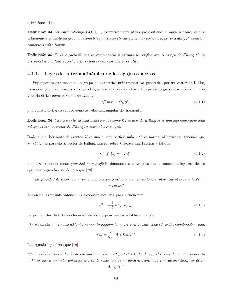
definiciones [14]:
Definicion 34 Un espacio-tiempo (M, gµν), asintoticamente plano que contiene un agujero negro, se dice
estacionario si existe un grupo de isometrıas uniparametricas generadas por un campo de Killing ξµ asintoti-
camente de tipo tiempo.
Definicion 35 Si un espacio-tiempo es estacionario y ademas se verifica que el campo de Killing ξµ es
ortogonal a una hipersuperficie Σ, entonces decimos que es estatico.
4.1.1. Leyes de la termodinamica de los agujeros negros
Supongamos que tenemos un grupo de isometrıas uniparametricas generadas por un vector de Killing
rotacional φµ; en este caso se dice que el agujero negro es axisimetrico. Un agujero negro estatico o estacionario
y axisimetrico posee el vector de Killing
ξµ = tµ + ΩHφµ, (4.1.1)
y la constante ΩH se conoce como la velocidad angular del horizonte.
Definicion 36 Un horizonte, al cual denotaremos como K, se dice de Killing si es una hipersuperficie nula
tal que existe un vector de Killing ξµ normal a este. [16]
Dado que el horizonte de eventos H es una hipersuperficie nula y ξµ es normal al horizonte, tenemos que
∇µ (ξνξν) es paralela al vector de Killing. Luego, sobre H existe una funcion κ tal que
∇µ (ξνξν) = −2κξµ, (4.1.2)
donde κ se conoce como gravedad de superficie, dandonos la clave para dar a conocer la ley cero de los
agujeros negros la cual declara que [79]
“La gravedad de superficie κ de un agujero negro estacionario es uniforme sobre todo el horizonte de
eventos.”
Asimismo, es posible obtener una expresion explıcita para κ dada por
κ2 = −1
2∇µξν∇µξν . (4.1.3)
La primera ley de la termodinamica de los agujeros negros establece que [79]
“La variacion de la masa δM , del momento angular δJ y del area de superficie δA estan relacionados como
δM =κ
8πδA+ ΩHδJ.” (4.1.4)
La segunda ley afirma que [79]
“Si se satisface la condicion de energıa nula, esto es Tµνkµkν ≥ 0 donde Tµν el tensor de energıa-momento
y kµ es un vector nulo, entonces el area de superficie de un agujero negro nunca puede disminuir, es decir
δA ≥ 0 .”
84
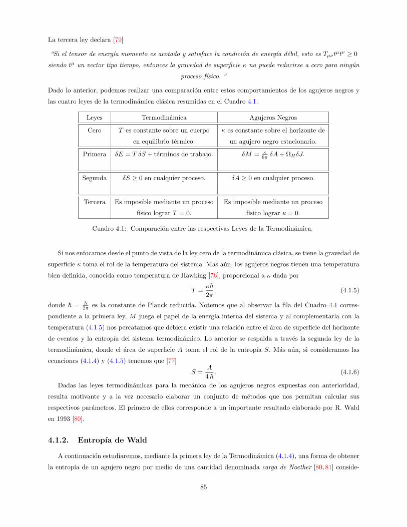
La tercera ley declara [79]
“Si el tensor de energıa momento es acotado y satisface la condicion de energıa debil, esto es Tµνtµtν ≥ 0
siendo tµ un vector tipo tiempo, entonces la gravedad de superficie κ no puede reducirse a cero para ningun
proceso fısico. ”
Dado lo anterior, podemos realizar una comparacion entre estos comportamientos de los agujeros negros y
las cuatro leyes de la termodinamica clasica resumidas en el Cuadro 4.1.
Leyes Termodinamica Agujeros Negros
Cero T es constante sobre un cuerpo κ es constante sobre el horizonte de
en equilibrio termico. un agujero negro estacionario.
Primera δE = T δS + terminos de trabajo. δM = κ8π δA+ ΩHδJ.
Segunda δS ≥ 0 en cualquier proceso. δA ≥ 0 en cualquier proceso.
Tercera Es imposible mediante un proceso Es imposible mediante un proceso
fısico lograr T = 0. fısico lograr κ = 0.
Cuadro 4.1: Comparacion entre las respectivas Leyes de la Termodinamica.
Si nos enfocamos desde el punto de vista de la ley cero de la termodinamica clasica, se tiene la gravedad de
superficie κ toma el rol de la temperatura del sistema. Mas aun, los agujeros negros tienen una temperatura
bien definida, conocida como temperatura de Hawking [76], proporcional a κ dada por
T =κ~2π, (4.1.5)
donde ~ = h2π es la constante de Planck reducida. Notemos que al observar la fila del Cuadro 4.1 corres-
pondiente a la primera ley, M juega el papel de la energıa interna del sistema y al complementarla con la
temperatura (4.1.5) nos percatamos que debiera existir una relacion entre el area de superficie del horizonte
de eventos y la entropıa del sistema termodinamico. Lo anterior se respalda a traves la segunda ley de la
termodinamica, donde el area de superficie A toma el rol de la entropıa S. Mas aun, si consideramos las
ecuaciones (4.1.4) y (4.1.5) tenemos que [77]
S =A
4 ~. (4.1.6)
Dadas las leyes termodinamicas para la mecanica de los agujeros negros expuestas con anterioridad,
resulta motivante y a la vez necesario elaborar un conjunto de metodos que nos permitan calcular sus
respectivos parametros. El primero de ellos corresponde a un importante resultado elaborado por R. Wald
en 1993 [80].
4.1.2. Entropıa de Wald
A continuacion estudiaremos, mediante la primera ley de la Termodinamica (4.1.4), una forma de obtener
la entropıa de un agujero negro por medio de una cantidad denominada carga de Noether [80, 81] conside-
85
rando teorıas gravitatorias covariantes, esto es, aquellas teorıas invariantes ante difeomorfismos. Asimismo,
tendremos un Lagrangiano L(φ) definido sobre una variedad (M, gµν) orientada de dimension D, donde φ
representa a la metrica gµν , otros campos de materia ψ y sus derivadas. Dado que el Lagrangiano L(φ) posee
esta invariancia, por hipotesis, de acuerdo a [81] lo podemos reexpresar de la forma
L = L(gµν ,∇µ1Rνσρτ , . . . ,∇(µ1
. . .∇µm)Rνσρτ , ψ, . . . ,∇(µ1. . .∇µl)ψ
), (4.1.7)
donde ∇ denota la derivada covariante asociada al tensor gµν y Rνσρτ es la curvatura de gµν . Si variamos el
Lagrangiano L respecto a φ tenemos que
δL = E(φ)δφ+ dΘ(φ, δφ). (4.1.8)
Usualmente, y como veremos luego, la ecuacion (4.1.8) se obtiene por medio de la accion de la teorıa
gravitatoria donde Θ es un termino de superficie que no afecta en las ecuaciones de movimiento. Por otro
lado, tenemos que
LξL =∂L
∂φLξφ = d (ξ · L) , (4.1.9)
donde L corresponde a la derivada de Lie a lo largo del campo de Killing ξ y la operacion · denota la
contraccion del ındice del vector ξ con el primer ındice de la forma diferencial L. Combinando las ecuaciones
(4.1.8) y (4.1.9) tenemos una expresion para la corriente de Noether J de la forma
J = Θ (φ,Lξφ)− ξ · L, (4.1.10)
donde
dJ = −E(φ)Lξφ. (4.1.11)
Notemos que J es una cantidad conservada si se satisfacen las ecuaciones de movimiento E(φ) = 0. Dado
lo anterior, obtenemos una forma diferencial Q localmente construida a partir de φ y ξµ, siempre que φ
satisfaga E(φ) = 0, conocida como carga de Noether, satisfaciendo
J = dQ. (4.1.12)
Ahora definamos la (D − 1)-forma Ω en base a dos variaciones arbitrarias de los campos φ
Ω(φ, δ1φ, δ2φ) := δ2Θ(φ, δ1φ)− δ1Θ(φ, δ2φ), (4.1.13)
y calculemos la variacion de la corriente J como
δJ = δΘ (φ,Lξφ)− ξ · δL = δΘ (φ,Lξφ)− LξΘ(φ, δφ) + d(ξ ·Θ(φ, δφ)
). (4.1.14)
Aquı hemos utilizado la ecuacion (4.1.8) junto con E(φ) = 0, ademas de la identidad sobre la derivada de
Lie para una forma diferencial µ [81]
Lξµ = ξ · dµ+ d (ξ · µ) . (4.1.15)
Observemos que la ecuacion (4.1.14) la podemos reescribir como
Ω(φ, δφ,Lξφ) = δJ− d(ξ ·Θ(φ, δφ)
), (4.1.16)
86
entregando una estructura para definir el Hamiltoniano H para posteriormente integrar sobre una hipersu-
perficie de Cauchy Σ. En efecto, ante una variacion de los campos φ, la variacion del Hamiltoniano esta dada
por
δH =
∫
Σ
Ω(φ, δφ,Lξφ) =
∫
Σ
[δJ− d
(ξ ·Θ(φ, δφ)
)]=
∫
Σ
[δdQ− d
(ξ ·Θ(φ, δφ)
)], (4.1.17)
donde hemos utilizado la expresion (4.1.12) en el lado izquierdo de la ecuacion (4.1.17). Si δφ satisface las
ecuaciones de movimiento linealizadas, entonces podemos conmutar el operador derivativo y la variacion δ
transformando δH de la forma
δH =
∫
Σ
d[δQ−
(ξ ·Θ(φ, δφ)
)]. (4.1.18)
Para lo siguiente, debemos introducir una nueva definicion [82]:
Definicion 37 Un horizonte de Killing bifurcado corresponde a un par de hipersuperficies nulas Kµ y Kνque se intersectan en una superficie de dimension (D − 2) de tipo espacio S, conocida como superficie de
bifurcacion, de tal manera que Kµ y Kν son horizontes de Killing respecto al mismo campo de Killing ξµ.
Suponiendo un horizonte de Killing bifurcado C, con ξ normal al horizonte de eventos e integrando la
expresion (4.1.18), obtenemos que
δH∞ = δ
∫
CQ, (4.1.19)
utilizando el hecho que el vector de Killing ξ se anula en C. La magnitud H∞ corresponde a la energıa
canonica conjugada asociada al vector ξ cuando el espacio-tiempo es asintoticamente plano. Si el vector de
Killing toma la forma particular dada en (4.1.1), entonces tenemos
δH∞ = δM − ΩHδJ, (4.1.20)
donde se muestra en [81] que
δ
∫
CQ =
κ
2πδS, (4.1.21)
siendo κ la gravedad superficial. Finalmente, podemos escribir la entropıa de Wald SW de la forma
SW = −2π
∫
C
δL
δRµνσρεµνεσρ. (4.1.22)
Aquı εµν corresponde a un vector binormal a C, antisimetrico y normalizado de la forma εµνεµν = −2,
el Lagrangiano L se considera como una densidad escalar y su derivada se obtiene tomando el tensor de
Riemann Rµνσρ como un campo independiente de la metrica gµν .
Si bien el metodo de Wald es un metodo poderoso para calcular la entropıa S de soluciones de agujeros
negros, necesitamos procedimientos que nos permitan obtener la masa (energıa) asociada a estas mismas
soluciones para ası, junto con la temperatura dada en (4.1.5), ser consistentes con la primera ley de la
termodinamica (4.1.4). A continuacion estudiaremos algunos de estos procedimientos, desde el formalismo
ADM [83] hasta un metodo reciente conocido como formalismo cuasilocal [92].
4.1.3. Formalismos para obtener la masa de soluciones de agujeros negros
Como un primer acercamiento expondremos el metodo ADM, cuya base consiste en reescribir la accion
(2.2.13) en terminos de una metrica puramente espacial hij , ademas de una funcion N denominada lapso
87
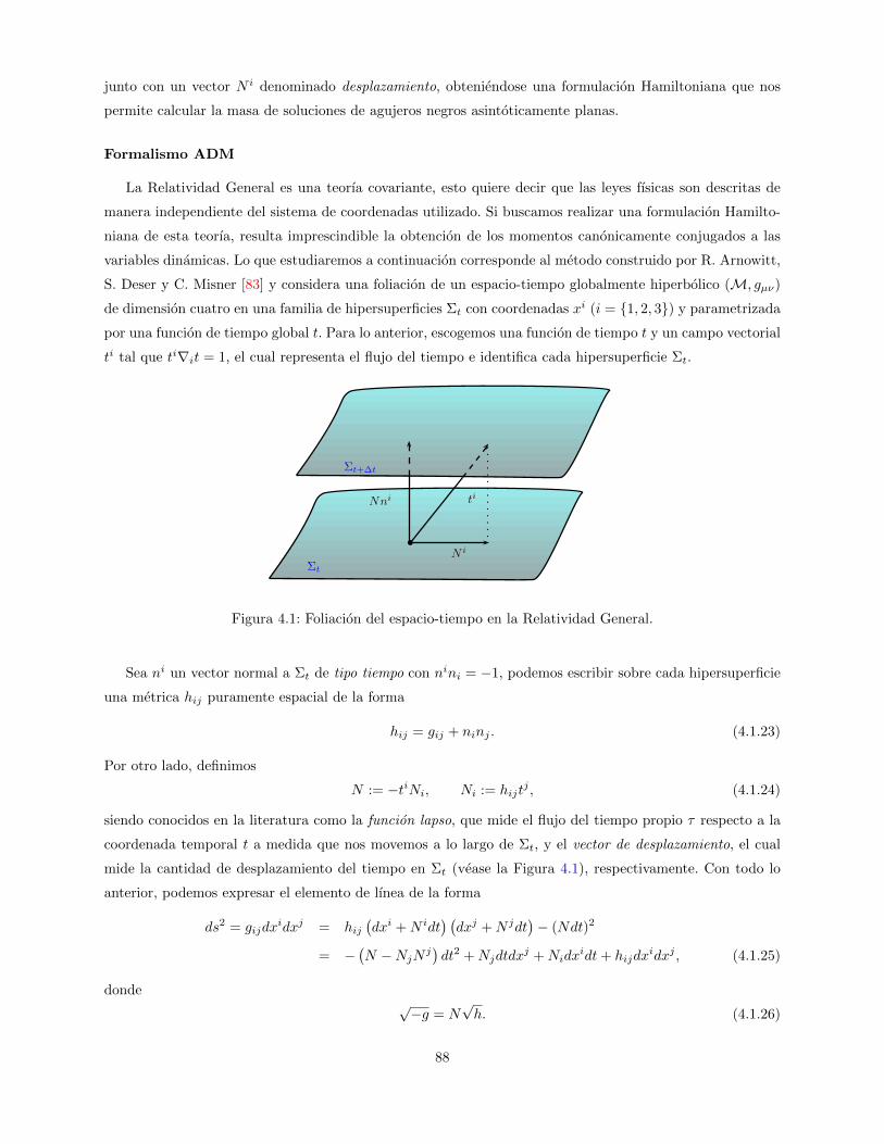
junto con un vector N i denominado desplazamiento, obteniendose una formulacion Hamiltoniana que nos
permite calcular la masa de soluciones de agujeros negros asintoticamente planas.
Formalismo ADM
La Relatividad General es una teorıa covariante, esto quiere decir que las leyes fısicas son descritas de
manera independiente del sistema de coordenadas utilizado. Si buscamos realizar una formulacion Hamilto-
niana de esta teorıa, resulta imprescindible la obtencion de los momentos canonicamente conjugados a las
variables dinamicas. Lo que estudiaremos a continuacion corresponde al metodo construido por R. Arnowitt,
S. Deser y C. Misner [83] y considera una foliacion de un espacio-tiempo globalmente hiperbolico (M, gµν)
de dimension cuatro en una familia de hipersuperficies Σt con coordenadas xi (i = 1, 2, 3) y parametrizada
por una funcion de tiempo global t. Para lo anterior, escogemos una funcion de tiempo t y un campo vectorial
ti tal que ti∇it = 1, el cual representa el flujo del tiempo e identifica cada hipersuperficie Σt.
Σt+∆t
N i
Nni ti
Σt
Figura 4.1: Foliacion del espacio-tiempo en la Relatividad General.
Sea ni un vector normal a Σt de tipo tiempo con nini = −1, podemos escribir sobre cada hipersuperficie
una metrica hij puramente espacial de la forma
hij = gij + ninj . (4.1.23)
Por otro lado, definimos
N := −tiNi, Ni := hijtj , (4.1.24)
siendo conocidos en la literatura como la funcion lapso, que mide el flujo del tiempo propio τ respecto a la
coordenada temporal t a medida que nos movemos a lo largo de Σt, y el vector de desplazamiento, el cual
mide la cantidad de desplazamiento del tiempo en Σt (vease la Figura 4.1), respectivamente. Con todo lo
anterior, podemos expresar el elemento de lınea de la forma
ds2 = gijdxidxj = hij
(dxi +N idt
) (dxj +N jdt
)− (Ndt)2
= −(N −NjN j
)dt2 +Njdtdx
j +Nidxidt+ hijdx
idxj , (4.1.25)
donde√−g = N
√h. (4.1.26)
88
El segundo paso a estudiar correponde a reexpresar el Lagrangiano
L =√−g(4)
R, (4.1.27)
en terminos de (hij , N,Ni). Para ello, podemos obtener [14]
Gijninj =
1
2
((3)R−KijK
ij +K2), (4.1.28)
Rijninj = K2 −KijK
ij −∇i(ni∇jnj
)+∇j
(ni∇inj
), (4.1.29)
donde los dos ultimos terminos de (4.1.29) son terminos de frontera y los descartamos en este caso en
particular, mientras que Kij es la curvatura extrınseca sobre Σt definida como
Kij := hki hlj∇knl =
1
2Lnhij =
1
2N−1 (Lthij − LNhij) =
1
2N−1
(hij −DiNj −DjNi
). (4.1.30)
Aquı Ln corresponde a la derivada de Lie a lo largo del vector n y el operador Di es el operador derivada
sobre Σt asociado con hij , esto es
DcTa1...ak
b1...bl = ha1d1 . . . h
akdkh
e1b1 . . . h
elblh
fc∇fT d1...dk
e1...el . (4.1.31)
Ademas, podemos expresar la curvatura escalar de la forma
R = 2(Gijn
inj −Rijninj), (4.1.32)
y junto con las ecuaciones (4.1.28) y (4.1.29) podemos expresar el Lagrangiano (4.1.27) como
L = N√h(
(3)R+KijKij −K2
),
= N√h[
(3)R+(hilhjm − hijhlm
)KijKlm
], (4.1.33)
donde
∂L
∂hij=
∂L
∂Lthij=√h(Kij −Khij
), πN =
∂L
∂N= 0, πiN =
∂L
∂Ni= 0, (4.1.34)
y la densidad Hamiltoniana H queda de la forma
H = πij hij − L
= −√h[N(
(3)R−KijKij +K2
)+ 2
(Khji −Kj
i
)DjN
i]
= −√h[N(
(3)R−KijKij +K2
)− 2N i
(DiK −DjK
ji
)]− 2√hDj
(KN j −Kj
iNi).(4.1.35)
Notemos que el ultimo termino de (4.1.35) es un termino de frontera y, como antes, lo descartamos para este
analisis. Finalmente, tenemos que el Hamiltoniano viene dado por la expresion
H = −∫
Σt
(N c0 − 2N i ci
)√hd3y, (4.1.36)
donde
c0 = (3)R−KijKij +K2, ci = DiK −DjK
ji . (4.1.37)
89

Ahora debemos modificar convenientemente la accion de Einstein-Hilbert para que este bien definida al
considerar soluciones asintoticamente planas. Concretamente, analizaremos una expresion de la forma [79,84]
S =1
16πG
∫
V
d4x√−g(4)R+
1
8πG
∮
∂V
d3y√h(Y − Y0), (4.1.38)
donde ∂V corresponde a la frontera del dominio V , Y es la traza de la curvatura extrınseca de ∂V embebida
en (M, gij) e Y0 es la curvatura extrınseca de ∂V embebida en (M, γij), donde γij es una metrica Lorentziana
sobreM que es plana en ∂V . Adicionalmente,√hd3y es el elemento de volumen inducido por gij sobre ∂V ,
mientras que hij es la metrica inducida sobre la hipersuperficie ∂V y h su respectivo determinante [85].
Definamos lo siguiente
St := ∂V ∩ Σt, (4.1.39)
donde asumiremos que este conjunto tiene la topologıa de una esfera. Su respectivo Hamiltoniano gravi-
tacional derivado de la accion (4.1.38) contiene un termino adicional al calculado en (4.1.36) expresado
como [84]
H ′ = − 1
16πG
∫
Σ′t
(N c0 − 2N i ci
)√hd3y − 1
8πG
∮
Std2z√q[N (k − k0)−Ni
(Kij −Khij
)sj], (4.1.40)
donde Σ′t es una seccion de Σt acotada por St, k corresponde a la traza de la curvatura extrınseca de Stembebida en (Σt, hij) y k0 a la traza de la curvatura extrınseca de St embebida en (Σt, fij), siendo fij
una metrica plana obtenida asintoticamente de hij . Asimismo, si es un vector unitario normal a St en Σt
y d2z√q es el elemento de superficie inducido por la metrica del espacio-tiempo sobre St, siendo qij la
respectiva metrica inducida y q su determinante.
Por otro lado, para soluciones de las ecuaciones de Einstein se tiene que
c0 = 0 y ci = 0, ∀i, (4.1.41)
de modo que (4.1.40) toma la forma
H ′sol = − 1
8πG
∮
Std2z√q[N (k − k0)−Ni
(Kij −Khij
)sj]. (4.1.42)
La energıa total contenida en la hipersuperficie Σt es definida como un valor numerico de (4.1.42) tomando
St y llevandolo al infinito espacial, con coordenadas (t, xi) tal que N = 1 y Ni = 0,∀i [85]. Finalmente, la
masa ADM viene dada por
MADM := − 1
8πGlımSt→∞
∮
Std2z√q (k − k0) , (4.1.43)
la cual podemos reescribirla como
MADM =1
16πGlımSt→∞
∮
Std2z√q[Djhij −Di
(fklhkl
)]si, (4.1.44)
donde Di corresponde a la conexion asociada a la metrica fij . Si trabajamos en coordenadas cartesianas (xi)
con
Di =∂
∂xi, fij = δij , (4.1.45)
la expresion (4.1.44) se convierte finalmente en
MADM =1
16πGlımSt→∞
∮
Std2z√q
(∂hij∂xj
− ∂hjj∂xi
)si. (4.1.46)
90

Formalismo ADT
Si bien el formalismo ADM es bueno para agujeros negros asintoticamente planos (tales como por ejem-
plo la solucion de Schwarzschild), se ha mostrado que es insuficiente para espacio-tiempos mas genericos.
Otro metodo que estudiaremos corresponde al procedimiento elaborado por L. Abbott, S. Deser y B. Te-
kin conocido como el formalismo ADT [86–88], el cual originalmente define cantidades conservadas para
espacio-tiempos cuyo comportamiento asintotico es de curvatura constante.
Consideremos en primer lugar las siguientes ecuaciones:
Eµν = κ τµν , (4.1.47)
donde Eµν es el tensor de Einstein para una accion gravitatoria local, τµν describe la fuente de materia y κ
es una constante de acoplamiento. Podemos linealizar la metrica gµν de la forma
gµν = gµν + hµν , (4.1.48)
y supondremos que gµν es la metrica base satisfaciendo Eµν(g) = 0 para τµν = 0, mientras que el tensor hµν
debera desvanecerse al infinito [86]. Linealizando la expresion (4.1.47) se obtiene
δEµν := ELµν = κTµν . (4.1.49)
Aquı, δEµν es lineal respecto a hµν y el nuevo tensor Tµν contiene todas las ecuaciones referentes a la parte
no lineal, ası como tambien al tensor τµν . Es importante notar que tanto la derivada covariante como la
operacion de subir y bajar ındices se realizan con respecto a la metrica base. Si suponemos ademas que la
metrica gµν admite un conjunto de vectores de Killing ξµ que satisfacen
∇µξν + ∇ν ξµ = 0, (4.1.50)
junto con
∇µTµν = 0, (4.1.51)
obtenemos la expresion
∇µ(δEµν ξν
)= 0 = ∂µ
(√−g δEµν ξν). (4.1.52)
De lo anterior podemos construir una corriente conservada, conocida en la literatura como corriente ADT,
mediante la contraccion de las ecuaciones de movimiento linealizadas δEµν y un vector de Killing ξν . Asi-
mismo, de esta corriente se define un potencial antisimetrico Qµν tal que
Jµ := δEµν ξν = ∇νQµν , (4.1.53)
Finalmente, la carga conservada toma la forma
Qµ(ξ) =
∫
Σ
dD−1x√−g δEµν ξν =
∮
∂Σ
dD−2x dSν Qµν , (4.1.54)
donde Σ denota la hipersuperficie de dimension (D − 1) de un espacio-tiempo de dimension D y ∂Σ es su
frontera, de dimension (D − 2), con elemento de superficie dS.
91

Debido a que la carga conservada depende de la teorıa, como ejemplo practico consideraremos las ecua-
ciones de Einstein junto con una constante cosmologica (3.0.4) sin una fuente de materia. La metrica base
gµν es tomada como el espacio-tiempo de curvatura constante, ello implica que el tensor de Riemann, tensor
de Ricci y escalar de Ricci vienen dados por (3.0.1), (3.0.5) y (3.0.6) respectivamente.
La linealizacion de las ecuaciones de movimiento (3.0.4) nos permiten obtener
G(L)µν −
2Λ
D − 2hµν = κTµν , (4.1.55)
donde G(L)µν = R
(L)µν − 1
2R(L)gµν y
R(L)µν =
1
2
(∇σ∇µhνσ + ∇σ∇νhµσ − hµν − ∇µ∇νh
), (4.1.56)
R(L) = −h+ ∇σ∇µhσµ −2Λ
D − 2h. (4.1.57)
Utilizando las ecuaciones (4.1.56) y (4.1.57), ademas de la inclusion de un vector de Killing ξµ y reordenando
los terminos, tenemos que la parte izquierda de la ecuacion (4.1.55) se convierte en
2Gµν(L)ξν −4Λ
D − 2hµν ξν = ∇ρQµρ, (4.1.58)
donde
Qµρ = ξν∇µhρν − ξν∇ρhµν + ξµ∇ρh− ξρ∇µh+ hµν∇ρξν − hρν∇µξν + ξρ∇νhµν
−ξµ∇νhρν + h∇µξρ, (4.1.59)
y la carga conservada para a ser la expresion (4.1.54), donde la conservacion de la corriente esta garantizada
por la propiedad de antisimetrıa del tensor Qµρ [89].
Si consideramos ahora un ambiente asintoticamente plano, donde no hay una contribucion de la constante
cosmologica Λ, obtenemos la masa ADM en terminos de coordenadas cartesianas en dimension D arbitra-
ria [88], la cual para el caso tetradimensional corresponde al resultado obtenido previamente en (4.1.46).
Asimismo, los autores en [88] calculan la masa para la solucion de Schwarzschild-AdS [90] dada en (3.3.2)
con γ = 1, y extienden el metodo para teorıas gravitatorias asociadas a curvaturas cuadraticas en D dimen-
siones.
Una condicion de este metodo es el hecho que la metrica base debe satisfacer las ecuaciones de movimiento
(4.1.47) en el vacıo. Sin embargo, en [89, 91] proponen una extension del metodo ADT, el cual linealiza la
metrica sobre una base gµν arbitraria, permitiendo calcular tanto la masa como el momento angular para
las teorıas conocidas como gravedad masiva topologica y nueva gravedad masiva, que seran estudiadas en la
seccion 4.2. El resultado es el siguiente:
JµADT := ∇νQµνADT = δEµν ξν + Eµσhσν ξν −1
2ξµEρσhρσ +
1
2ξν Eµν h, (4.1.60)
donde recuperamos la corriente original (4.1.53) cuando imponemos la condicion Eµν(g) = 0. De la misma
manera, podemos reescribir la ecuacion (4.1.60) de la forma [92]
δ(√−gEµν ξν
)− 1
2
√−gξµEαβhαβ = ∂ν(√−g QµνADT
). (4.1.61)
92

Formalismo cuasilocal
Otro metodo para calcular la masa de soluciones de agujeros negros corresponde a una generalizacion
cuasilocal del formalismo ADT estudiado anteriormente, donde no es necesario descomponer la metrica gµν
de la forma (4.1.48), ademas de simplificar sustancialmente los calculos [92,93].
Comencemos considerando una teorıa covariante de la gravedad para un espacio-tiempo de dimension D
S[gµν ] =1
κ
∫dDx√−gL[gµν , R,Rµν , Rµνσρ,∇R, . . .], (4.1.62)
la cual no incluye campos asociados a una fuente de materia y κ es una constante de acoplamiento. La
variacion de la accion (4.1.62) respecto a la metrica nos permite obtener
δS =1
κ
∫dDx
[√−g Eµνδgµν + ∂µΘµ(g, δg)], (4.1.63)
donde Eµν = 0 es la expresion para las ecuaciones de movimiento y Θµ(g, δg) es un termino de superficie.
Tomando en cuenta un difeomorfismo ζ, la metrica se transforma en
δζgµν = 2∇(µζν), (4.1.64)
mientras que el cambio de la densidad Lagrangiana es dado por
δζ(√−gL
)= ∂µ
(ζµ√−gL
). (4.1.65)
Si agregamos la identidad de Bianchi del tensor Eµν , esto es ∇µEµν = 0, logramos obtener una corriente
conservada fuera de la cascara (en el sentido que no estamos utilizando las ecuaciones de movimiento Eµν = 0)
de la forma
∂µ[2√−g Eµν(g)ζν + ζµ
√−gL(g)−Θµ(g; ζ)]
= ∂µJµ(g; ζ) = 0, (4.1.66)
donde podemos introducir un tensor antisimetrico Kµν , denominado potencial de Noether fuera de la cascara,
tal que Jµ := ∂νKµν .
Ahora, el objetivo es mostrar el vınculo entre el potencialKµν y el potencial correspondiente a la extension
del metodo ADT expuesto en (4.1.61), donde omitiremos la notacion de barras. Para ello, el difeomorfismo
ζ sera tomado como un vector de Killing ξ y trabajaremos en el cambio del potencial de Noether bajo
la variacion de la metrica, esto es δKµν , preservando el vector de Killing: δξµ = 0. Dada esta variacion,
podemos escribir el cambio de la corriente Jµ en terminos del potential Kµν como
∂ν (δKµν) = 2 δ(√−gEµνξν
)+ ξµδ
(√−gL)− δΘµ(g; ξ). (4.1.67)
Dado que hemos asumido δξµ = 0, podemos utilizar la siguiente relacion sobre el termino de superficie [81]
LξΘµ(g; δg) = δΘµ(g; ξ), (4.1.68)
donde Lξ representa la derivada de Lie a lo largo del vector de Killing ξ, mientras que el termino de la
derecha corresponde a la variacion respecto a la metrica. Con todo lo anterior, las ecuaciones (4.1.61),
(4.1.67) y (4.1.68) permiten obtener
√−g QµνADT (g, δg) =1
2δKµν(g; ξ)− ξ[µΘν](g, δg). (4.1.69)
93

Esta expresion es clave, pues permite formular una carga conservada en terminos del potencial de Noether
Kµν , el vector de Killing ξµ y de Θµ. En [92,93], los autores proponen incorporar un camino uniparametrico
dentro del espacio solucion, caracterizado por una constante s ∈ [0, 1]. Este camino es tomado como una
interpolacion mediante un parametro libre C dentro de las soluciones de las ecuaciones de movimiento, de
tal manera que sC ∈ [0, C]. Sobre la base del potencial QµνADT dado en (4.1.69), podemos obtener la carga
conservada cuasilocal de la forma
Q(ξ)=1
κ
∫
BdD−2xµν
(∆Kµν(ξ)− 2ξ[µ
∫ 1
0
ds Θν]), (4.1.70)
donde ∆Kµν(ξ) = Kµνs=1(ξ)−Kµν
s=0(ξ) corresponde a la diferencia finita entre dos puntos finales del camino,
mientras que dD−2xµν representa la integracion sobre un subespacio de codimension dos y B es una region
finita del espacio-tiempo que no necesita ser localizada en el infinito asintotico [93].
De manera concreta, consideremos el caso de una teorıa que posea correcciones de curvaturas superiores,
esto es L = L[g,R,R2, RµνRµν , · · · ]. Notemos que las ecuaciones de movimiento respecto a la metrica Eµνtoman la forma [92]
Eµν = P αβγ(µ Rν)αβγ − 2∇ρ∇σPµνρσ −
1
2gµνL, (4.1.71)
donde Pµνρσ = ∂L/∂Rµνρσ. Ademas, el termino de superficie y el potencial de Noether son dados por [93]
Θµgrav(δg) = 2
√−g[Pµ(αβ)γ∇γδgαβ − δgαβ∇γPµ(αβ)γ
], (4.1.72)
Kµνgrav =
√−g [2Pµνρσ∇ρξσ − 4ξσ∇ρPµνρσ]. (4.1.73)
Este caso particular de teorıas son sumamente importantes cuando se analizan soluciones de agujeros negros
asintoticamente Lifshitz. Mas aun, en [74,75] los autores encuentran interesantes familias de estas soluciones
considerando correcciones de curvaturas cuadraticas a la gravedad de Einstein, donde en [94, 95] extienden
este estudio mediante el calculo de sus respectivas masas utilizando el metodo ADT, no logrando satisfacer
la primera ley de la termodinamica. No obstante, en [93] logran calcular la expresion asociada a la masa
para el agujero negro de Lifshitz tridimensional [74], ası como tambien para un caso particular de solucion en
cinco dimensiones [75] por medio de las ecuaciones (4.1.70 - 4.1.73). Lo interesante y motivante a la vez, es
el hecho que estos nuevos resultados son consistentes con la primera ley, lo cual nos permite abrir un camino
para estudiar nuevas teorıas gravitatorias, teniendo como pilar fundamental este formalismo cuasilocal.
4.2. Teorıas gravitatorias masivas
En el capıtulo 2 estudiamos la estructura de la teorıa de la Relatividad General de Einstein, donde
la geometrıa del espacio-tiempo esta determinada por una fuente de materia y la dinamica de esta fuente
esta establecida por esta misma geometrıa. No obstante, observaciones de supernovas [96–99] y su consecuen-
cia en la expansion acelerada del universo, sumado a la motivacion de conciliar la Relatividad General con la
Mecanica Cuantica, han llevado a intentar modificar las ecuaciones de Einstein en su estado puro [98]. Mas
aun, desde la perspectiva cuantica, la Relatividad General se puede considerar como una interaccion debil
de una partıcula, asociada a los grados de libertad, sin masa de spin-2 denominada graviton, [97, 98, 100],
94
donde modificar la gravedad significa necesariamente cambiar estos grados de libertad. Por ejemplo, en cua-
tro dimensiones, al incluir un pequeno termino de masa a la accion de Einstein-Hilbert (2.2.13) los grados
de libertad aumentan de dos a cinco.
4.2.1. Accion de Fierz-Pauli
En esta parte estudiaremos la accion asociada a una partıcula masiva en un espacio-tiempo plano, trans-
portada por un tensor simetrico hµν , conocida como la accion de Fierz-Pauli. En D-dimensiones, viene dada
por [97,101,102]
S =
∫dDx
[−1
2∂λhµν∂
λhµν + ∂µhνλ∂νhµλ − ∂µhµν∂νh+
1
2∂λh∂
λh− 1
2m2(hµνh
µν − h2)], (4.2.1)
donde h = ηµνhµν es la traza de la metrica, con ηµν la metrica del espacio-tiempo plano. La segunda
parte de la accion corresponde al termino de Pauli-Fierz masivo, siendo m el parametro de masa respectivo.
Adicionalmente, la expresion asociada a los terminos derivativos del tensor hµν son elegidos de tal manera que
al imponer m = 0, obtenemos la accion de Einstein-Hilbert linealizada. Ahora, variando la accion respecto
a hµν tenemos que
hµν − ∂λ∂µhλν − ∂λ∂νhλµ + ηµν∂λ∂σhλσ + ∂µ∂νh− ηµνh−m2(hµν − ηµνh) = 0, (4.2.2)
donde := ∂µ∂µ. Si suponemos que el parametro de masa m es distinto de cero, actuando la ecuacion
anterior con ∂µ se obtiene que
∂µhµν = ∂νh, (4.2.3)
transformando las ecuaciones de movimiento (4.2.2) de la forma
hµν − ∂µ∂νh−m2(hµν − ηµνh) = 0. (4.2.4)
Al multiplicar la ecuacion anterior por hµν , obtenemos que h = 0, lo cual implica que ∂µhµν = 0. Luego,
tenemos que la ecuacion (4.2.2) se reduce a una expresion dada por
(−m2
)hµν = 0. (4.2.5)
El resultado anterior, ademas de las ecuaciones (4.2.3) y (4.2.4), nos permiten mostrar que esta accion describe
una partıcula de spin-2 masiva. Inversamente, vemos que las ecuaciones (4.2.3), (4.2.4) y (4.2.5) implican
las ecuaciones de movimiento (4.2.2) [97]. Adicionalmente, mediante las condiciones anteriores, podemos
obtener los grados de libertad. En efecto, si consideramos un espacio-tiempo de cuatro dimensiones, debido
a la metrica hµν tenemos inicialmente diez grados de libertad, reduciendose a seis mediante la condicion
∂µhµν = 0, los cuales complementado con h = 0 obtenemos una teorıa con cinco grados de libertad para una
partıcula tetradimensional de spin-2. De modo similar, podemos extender la accion (4.2.1) considerando un
espacio-tiempo curvo, en particular estudiaremos dos teorıas gravitatorias masivas las cuales se presentan en
un espacio-tiempo tridimensional.
95

4.2.2. Gravedad masiva topologica
La primera teorıa que estudiaremos en tres dimensiones corresponde a la denominada gravedad masiva
topologica (GMT) [103,104], su respectiva accion esta dada por
SGMT = − 1
2κ
(SEH +
1
µSCS
), (4.2.6)
donde µ es el parametro de masa, SEH es la accion de Einstein-Hilbert junto a la constante cosmologica Λ
SEH =
∫d3x√−g (R− 2Λ) , (4.2.7)
mientras que SCS corresponde a la accion de Chern-Simons gravitacional
SCS =1
2
∫d3x√−gελµνΓρλσ
(∂µΓσρν +
2
3ΓσµγΓγνρ
). (4.2.8)
Aquı, εαβγ es el tensor de Levi-Civita, el cual esta conectado al sımbolo de Levi-Civita de la forma εαβγ =
(1/√−g) εαβγ , g es el determinante de la metrica y los Γ’s corresponden a los sımbolos de Christoffel definidos
en (2.1.9). La variacion de (4.2.6) con respecto a la metrica nos permite obtener
Rµν −1
2Rgµν + Λgµν +
1
µCµν = 0, (4.2.9)
donde Cµν = ε σρµ ∇σ(Rβν − 1
4Rgρν) se conoce como el tensor de Cotton, el cual es simetrico (Cµν = Cνµ),
covariantemente conservado (∇µCµν = 0) y no posee traza (gµνCµν = 0). Multiplicando la ecuacion (4.2.9)
por gµν , obtenemos que la curvatura escalar es R = 6Λ, permitiendo reescribir las ecuaciones de movimiento
de la forma
Rµν − 2Λgµν +1
µε σρµ ∇σRρν = 0. (4.2.10)
A su vez, el tensor de Cotton en tres dimensiones tiene una ıntima relacion respecto a variedades conforme-
mente planas.
Definicion 38 Una variedad (M, gµν) se dice conformemente plana (localmente) si para cada punto p ∈M,
existe un entorno U ⊆ M y una metrica equivalente conforme ω2 gµν , donde ω es una funcion suave no
nula, tal que (U, ω2 gµν) es plana.
Si consideramos una variedad de dimension mayor a tres, una condicion necesaria y suficiente para que sea
conformemente plana es que el tensor de Weyl (2.1.27) sea nulo. Por otra parte, en tres dimensiones el tensor
de Riemann viene dado por
Rρσµν = 2Rρ[µgν]σ + 2Rσ[νgµ]ρ +Rgρ[νgµ]σ, (4.2.11)
donde T[µν] = 12 (Tµν − Tνµ) y, por consiguiente, tenemos que el tensor de Ricci contiene toda la informacion
sobre la curvatura de la variedad. Al utilizar la ecuacion (4.2.11) en la expresion del tensor de Weyl dada en
(2.1.27), para D = 3 tenemos que este se desvanece. No obstante, para el caso tridimensional, una variedad es
conformemente plana si y solo si el tensor de Cotton se desvanece. Adicionalmente, la inclusion del termino
topologico involucra derivadas de tercer orden en la metrica, junto con ser una teorıa unitaria [104], esto
es, libre de partıculas fantasmas (aquellas que poseen energıa cinetica negativa), lo que fundamenta el signo
incorrecto en la accion (4.2.6), y taquiones (poseen una masa al cuadrado negativa) [98].
96

Gravedad masiva topologica linealizada
Consideremos ahora linealizar la metrica como
gµν = gµν + hµν , (4.2.12)
donde gµν es una metrica base de curvatura constante. El tensor de Ricci, escalar de Ricci y el tensor de
Cotton linealizados son respectivamente [105–107]
R(L)µν =
1
2
(∇σ∇µhνσ + ∇σ∇νhµσ − hµν − ∇µ∇νh
), (4.2.13)
R(L) = −h+ ∇σ∇µhσµ − 2Λh, (4.2.14)
C(L)µν = ε σρ
µ ∇σ(R(L)ρν −
1
4R(L)gρν − 2Λhρν
), (4.2.15)
donde las operaciones de subir y bajar ındices, ası como tambien de la derivada covariante las realizamos
respecto a la metrica gµν . Las ecuaciones de movimiento linealizadas para (4.2.9) estan dadas por
G(L)µν − 2Λhµν +
1
µC(L)µν = 0, (4.2.16)
con G(L)µν = R
(L)µν − 1
2R(L)gµν . Multiplicando la expresion (4.2.16) por gµν , tenemos que R(L) = 0 y las
ecuaciones de movimiento se convierten en
(R(L)µν − 2Λhµν
)+
1
µε σρµ ∇σ
(R(L)ρν − 2Λhρν
)= 0. (4.2.17)
Adicionalmente, los autores en [105] definen el tensor hµν := hµν − gµνh y las ecuaciones (4.2.17) pasan a
ser ( +
2
`2
)(hµν +
1
µε σρµ ∇σhρν
)= 0. (4.2.18)
Asimismo, definen los siguientes tres operadores diferenciales DI ,DD y DM que conmutan mutuamente:
(DI/D
)σµ
:= δσµ ± `ε ρσµ ∇ρ,
(DM
)σµ
:= δσµ +1
µε ρσµ ∇ρ, (4.2.19)
donde tenemos que la ecuacion (4.2.18) puede escribirse como
(DIDDDMh
)µν
= 0, (4.2.20)
obteniendose tres ramas de soluciones:
(DMhM
)µν
:= hMµν +1
µε σρµ ∇σhMρν = 0,
(DDhD
)µν
:= hDµν − `ε σρµ ∇σhDρν = 0,
(DIhI
)µν
:= hIµν + `ε σρµ ∇σhIρν = 0. (4.2.21)
La primera solucion corresponde a gravitones masivos, mientras que las otras dos dan referencia a gravitones
sin masa moviendose hacia la derecha y hacia la izquierda respectivamente [105].
97

4.2.3. Nueva gravedad masiva
A continuacion estudiaremos una segunda teorıa gravitatoria masiva tridimensional conocida como nue-
va gravedad masiva (NGM), la cual es equivalente a la accion de Fierz-Pauli (unitaria) linealizada para
gravitones masivos libres de spin-2 [108]. De manera introductoria, consideremos la siguiente accion en
D-dimensiones
S[gµν ] =1
2κ
∫dDx√−g
[R+ β1R
2 + β2RµνRµν + β3
(RµνσρR
µνσρ − 4RµνRµν +R2
)], (4.2.22)
donde hemos agregado correcciones de curvaturas cuadraticas a la gravedad de Einstein con βi’s constantes
y κ una constante de acoplamiento. Una de las ventajas de esta teorıa es que adquiere renormalizabilidad,
propiedad que no posee la accion de Einstein-Hilbert en un estado puro. Sin embargo, la inclusion del termino
RµνRµν conlleva la la aparicion de un termino fantasma, y la teorıa pasa a ser no unitaria [98, 109, 110]. El
termino que acompana a la constante de acoplamiento β3 corresponde al termino de Gauss-Bonnet estudiado
en la seccion 3.2, donde su contribucion a la accion (4.2.22) depende de la dimension del espacio-tiempo. En
particular, si consideramos el caso D = 4, el termino de Gauss-Bonnet pasa a ser un termino de superficie,
por lo tanto, no contribuye a las ecuaciones de movimiento. Mientras que para D = 3, tenemos que este
termino desaparece. Si variamos la accion (4.2.22) obtenemos [98]
Rµν −1
2Rgµν +Kµν = 0, (4.2.23)
donde
Kµν = 2β1R
(Rµν −
1
4Rgµν
)+ (2β1 + β2)(gµν−∇µ∇ν)R+ 2β3 [RRµν − 2RµσνρR
σρ
+RµσρτRσρτν − 2RµσR
σν −
1
4gµν
(RτλσρR
τλσρ − 4RσρRσρ +R2
)]+ β1
(Rµν −
1
2Rgµν
)
+2β1
(Rµσνρ −
1
4gµνRσρ
)= 0, (4.2.24)
el cual contiene derivadas de cuarto orden respecto a la metrica. En particular, para la teorıa NGM existe
una relacion especial entre las constantes de acoplamiento β1 y β2, dada por β1 = − 38β2, de tal forma que la
traza de Kµν sea proporcional a esta combinacion lineal de R2 con RµνRµν , removiendo el modo de spin-0
que serıa un fantasma [97,108]. Con todo lo anterior, tenemos que la teorıa NMG esta dada por
SNGM = − 1
2κ
∫d3x√−g
[R− 2λ− 1
m2K
], (4.2.25)
donde
K = RµνRµν −3
8R2. (4.2.26)
El signo negativo se justifica debido a la unitariedad de la teorıa, m es un parametro de masa que acompana
a K y λ es una constante que no necesariamente corresponde a la constante cosmologica Λ. Las ecuaciones
de movimiento de (4.2.25) son [108,111]
Rµν −1
2Rgµν + λgµν −
1
2m2Kµν = 0, (4.2.27)
98
donde
Kµν = −1
2Rgµν −
1
2∇µ∇νR+ 2Rµν + 4RµσνρR
σρ − 3
2RRµν −RσρRσρgµν +
3
8R2gµν . (4.2.28)
Multiplicando (4.2.27) por la metrica inversa gµν y utilizando gµνKµν = K, obtenemos la expresion
m2(6λ−R)−K = 0,
ello implica que, para una solucion de las ecuaciones (4.2.27) con m 6= 0
R = 6λ⇔ K = 0.
Adicionalmente, si consideramos un espacio-tiempo maximalmente simetrico en tres dimensiones, donde
Rµσνρ = Λ(gµνgσρ − gµρgσν), Rµν = 2Λgµν , R = 6Λ, (4.2.29)
y Kµν = − 12Λ2gµν , se obtiene una relacion entre la constante λ, la constante cosmologica Λ y el parametro
de masa m de la forma
λ = Λ
(1− Λ
4m2
). (4.2.30)
Lo anterior implica que las ecuaciones (4.2.27) admiten una solucion si y solo si m2
λ ≥ 1. Dependiendo del
signo de m2 y la constante λ, podemos separar los casos en AdS3, dS3 o de Minkowski [111].
Nueva gravedad masiva linealizada
De manera analoga a la teorıa GMT, analizaremos las ecuaciones de movimiento (4.2.27) linealizadas
entorno a una metrica base de curvatura constante gµν , donde el tensor y escalar de Ricci linealizado
corresponden a las expresiones (4.2.13) y (4.2.14). Ademas, las restantes cantidades son las siguientes [111]
Rλ(L)ρνµ =
1
2gλσ(∇ν∇µhσρ + ∇ν∇ρhµσ − ∇ν∇σhµρ)− (µ↔ ν), (4.2.31)
(∇µ∇νR)(L) = ∇µ∇νR(L), (∇σ∇ρRµν)(L) = ∇σ∇ρR(L)µν − 2Λ∇σ∇ρhµν . (4.2.32)
Sustituyendo lo anterior en las ecuaciones de movimiento (4.2.27), obtenemos
G(L)µν + λhµν −
1
2m2K(L)µν = 0, (4.2.33)
donde
G(L)µν = R(L)
µν −1
2gµνR
(L) − 3Λhµν , (4.2.34)
K(L)µν = −1
2R(L)
µν −1
2∇µ∇νR(L) + 2R(L)
µν − 4Λhµν − 5ΛR(L)µν
+3
2ΛR(L)gµν +
19
2Λ2hµν . (4.2.35)
Tomando la traza de la ecuacion (4.2.34) obtenemos que R(L) = 0, transformando las ecuaciones de movi-
miento linealizadas como(
1 +5Λ
2m2
)(R(L)
µν − 2Λhµν)− m2
(R(L)µν − 2Λhµν) = 0. (4.2.36)
99

Asimismo, de la misma manera que el caso GMT, los autores en [111] definen el tensor h := hµν − gµνh,
obteniendose
hµν = hµν −1
2gµν h, R(L) = ∇µ∇ν hµν + Λh = 0, (4.2.37)
donde se concluye que ∇µhµν = 0, implicando que h = −2h = 0. Finalmente, la ecuacion (4.2.36) se convierte
en [−
(m2 +
5
2Λ
)] [− 2Λ
]hµν = 0. (4.2.38)
Lo que nos permite concluir la existencia de dos ramas de soluciones, la primera de ellas corresponde al
sector de gravitones masivos, mientras que la segunda esta asociada a gravitones sin masa [111].
4.3. Calculo de la masa de agujeros negros considerando el for-
malismo cuasilocal
Debido a la importancia del formalismo cuasilocal en esta tesis, resulta necesario dar a conocer algunos
ejemplos presentes en la literatura, donde para cada uno de ellos, mostraremos la masa Mcuasilocal (4.1.70), en-
tropıa de Wald SW (4.1.22) y temperatura de Hawking T (4.1.5) (con ~ = 1) respectivamente. Comenzaremos
el estudio considerando la siguiente accion
S[gµν ,Φ] =1
2κ
∫dDx√−g
( (1− κ ξΦ2
)R− 2Λ + β1R
2 + β2RαβRαβ + β3RαβµνR
αβµν)
+
∫dDx√−g
[− 1
2∂µΦ∂µΦ− U(Φ)
], (4.3.1)
donde la seccion gravitatoria corresponde a la accion de Einstein-Hilbert con una constante cosmologica Λ,
ademas de las correcciones de curvaturas cuadraticas mas generales en D-dimensiones y κ es una constante de
acoplamiento. Mientras que la fuente de materia incluye a un campo escalar no mınimamente acoplado junto
a un potential, estudiado previamente en el capıtulo 3. Para cada uno de estos ejemplos, se considerara un
ansatz metrico dado en (3.3.1) con γ = 0.
Por otro lado, dado que la accion (4.3.1) posee una fuente de materia, las ecuaciones expuestas en
(4.1.72) y (4.1.73) deben modificarse. Observemos que, siguiendo el procedimiento realizado en [92], tanto
el potencial de Noether como el termino de superficie de la primera lınea de la accion (4.3.1) mantienen la
misma estructura, donde el tensor Pαβγδ esta dado por
Pαβγδ =1
4
(1
κ− ξΦ2
)(gαγgβδ − gαδgβγ
)+β1
2κR(gαγgβδ − gαδgβγ
)
+β2
4κ
(gβδRαγ − gβγRαδ − gαδRβγ + gαγRβδ
)+β3
κRαβγδ. (4.3.2)
Ahora debemos encontrar la contribucion de la otra seccion correspondiente al termino cinetico usual del
campo escalar junto al potencial U(Φ). Aplicando el mismo formalismo, tenemos que el termino de superficie
total de la accion (4.3.1) adquiere la forma
Θµ(δg, δΦ) = Θµgrav(δg) + Θµ
mat(δΦ), (4.3.3)
100

donde
Θµmat(δΦ) =
√−g ∂L
∂ (∂µΦ)δΦ = −√−g gµν∂νΦ δΦ. (4.3.4)
De lo anterior, construimos la corriente conservada Jµmat como
Jµmat := −2Tµνξν + ξµ(−1
2∂σΦ∂σΦ− U(Φ)
)−Θµ
mat(δξΦ), (4.3.5)
donde δξ denota la variacion del campo escalar bajo difeomorfismo y es dado por
δξΦ = LξΦ = ξσ∇σξ, (4.3.6)
mientras que
Tµν =1
2
(∂µΦ∂νΦ− 1
2gµν∂σΦ∂σΦ− gµνU(Φ)
). (4.3.7)
Sin embargo, con todo lo anterior tenemos que la corriente Jµmat se desvanece trivialmente. Como resultado
final, tenemos que la expresion para el potencial de Noether total Kµν debe ser
Kµν = Kµνgrav, (4.3.8)
con Pαβγδ dado en (4.3.2).
Como primer ejemplo, estudiaremos el agujero negro encontrado en [62] con k = 2, sin una fuente de
materia. Su respectivo elemento de lınea esta dado por
ds20 = −
(r2
l2− Ml(D−5)/2
r(D−5)/2
)dt2 +
(r2
l2− Ml(D−5)/2
r(D−5)/2
)−1
dr2 +r2
l2dΣ2
D−2,0, (4.3.9)
donde M es una constante de integracion asociada a la masa. Asimismo, las constantes βi’s y cosmologica
adquieren la forma
Λ = − (D − 1) (D − 2)
4 l2, β1 = −1
4β2 = β3 =
l2
2 (D − 3) (D − 4). (4.3.10)
Mediante las formulas (4.1.22) y (4.1.5) para la entropıa y temperatura respectivamente, podemos notar que
SW =2π rD−2
h ΣD−2,0
lD−2κ, T =
(D − 1) rh8π l2
, rh = lM2
D−1 , (4.3.11)
donde rh denota la ubicacion del horizonte de eventos y ΣD−2,0 representa la contribucion finita de la
integracion (D − 2)-dimensional sobre las variables planares. De lo anterior, el potencial de Noether (4.3.8)
y el termino de superficie (4.3.3) son dados por
Krt =(D − 5) (D − 2)M2
2 l (D − 4)κ+
(D + 1)M
l (D − 4)κ
(rl
)D−12 − 4
r (D − 4)κ
(rl
)D, (4.3.12)
∫ M
0
dM Θr =(D − 2)M2
2 l (D − 4)κ− (D + 1)M
l (D − 4)κ
(rl
)D−12
. (4.3.13)
Esto implica que la masa Mcuasilocal de la solucion (4.3.9) para a ser
Mcuasilocal =(D − 2) rD−1
h ΣD−2,0
4κ lD, (4.3.14)
101
donde podemos verificar que la entropıa y temperatura (4.3.11) junto con la masa (4.3.14) satisfacen la
primera ley de la termodinamica (4.1.4).
El segundo ejemplo a analizar, si no consideramos una fuente de materia, corresponde a los resultados
encontrados en [75], logrando obtener las respectivas masas para las tres familias de agujeros negros asintoti-
camente Lifshitz [112], mostrando que satisfacen la primera ley (4.1.4). La primera familia de soluciones
esta dada para un rango del exponente dinamico z > 2−D, siendo descrita por el elemento de lınea
ds20 = −r
2z
l2z
(1− Ml(z+D−2)/2
r(z+D−2)/2
)dt2 +
l2
r2
(1− Ml(z+D−2)/2
r(z+D−2)/2
)−1
dr2 +r2
l2dΣ2
D−2,0, (4.3.15)
donde rh = lM2
z+D−2 . Aquı, las constantes de acoplamiento son parametrizadas de la forma
Λ =(D − 2)
4l2
(197D − 389)z4 + 4(19D2 − 200D + 325)z3 + (D − 2)
[2(5D2 − 73D + 356)z2
+ 4(D3 − 2D2 + 15D − 62)z + (D + 2)(D − 1)(D − 2)2]/
P4(z), (4.3.16)
β1 = l2
27z6 − 18(3D − 4)z5 + 3(19D2 − 168D + 356)z4 − 12(11D3 − 84D2 + 196D − 120)z3
− (D − 2)[(19D3 − 330D2 + 2052D − 3640)z2 + 2(3D4 − 30D3 + 124D2 − 536D + 1024)z
+ (D + 2)(D − 2)2(D2 − 4D + 36)]/(
2(D − 3)(D − 4)(z +D − 2)2P4(z)), (4.3.17)
β2 = −2l2[3z2 + (D + 2)(D − 2)
]9z4 − 6(3D − 4)z3 − 8(D2 − 10)z2 + 2(D3 − 4D2 + 32D − 80)z
− (D − 2)[D3 + 2D2 − 12(D − 2)
]/((D − 3)(D − 4)(z +D − 2)2P4(z)
), (4.3.18)
β3 = l2[3z2 + (D + 2)(D − 2)
]9z3 − 3(9D − 14)z2 − (D − 2)
[(5D − 62)z +D2 − 4D + 36
]
/(2(D − 3)(D − 4)(z +D − 2)P4(z)
), (4.3.19)
donde P4 es un polinomio de grado cuatro respecto al exponente dinamico z dado por
P4(z) = 27z4 − 4(27D − 45)z3 − (D − 2)[2(5D − 116)z2 + 4(D2 −D + 30)z + (D + 2)(D − 2)2
].
Para este caso, la masa Mcuasilocal, entropıa de Wald SW y la temperatura de Hawking T son
Mcuasilocal = (D − 2) ΣD−2,0
(rhl
)z+D−2[(
3 z2 +D2 − 4)
(D − 2 + 3 z) (3 z −D − 2)
4 lP4 (z)κ
], (4.3.20)
SW = 2πΣD−2,0
(rhl
)D−2[(
3 z2 +D2 − 4)
(D − 2 + 3 z) (3 z −D − 2)
P4 (z)κ
], (4.3.21)
T =(z +D − 2)
8πl
(rhl
)z. (4.3.22)
102

La segunda familia considera el caso z > 1, cuya solucion adquiere la forma
ds20 = −r
2z
l2z
(1− Ml2(z−1)
r2(z−1)
)dt2 +
l2
r2
(1− Ml2(z−1)
r2(z−1)
)−1
dr2 +r2
l2dΣ2
D−2,0, (4.3.23)
donde el horizonte se encuentra ubicado en rh = lM1
2(z−1) . Para esta situacion, la solucion (4.3.23) existe a
traves de la siguiente eleccion de las constantes de acoplamiento
Λ = − (z − 1)[z2 −Dz − (D − 1)(D − 2)
]
2l2(z −D), (4.3.24)
β1 = l2[3(D − 1)(D − 2)z3 − (2D3 − 2D2 − 11D + 20)z2 + (3D3 − 14D2 + 19D + 10)z
+ (D + 2)(D − 4)]/[
2(D − 2)(D − 3)(D − 4)z(z − 1)(z −D)(3z +D − 4)], (4.3.25)
β2 = −l2(D − 1)(2z −D − 2)[6(D − 2)z2 − (D2 − 3D + 8)z − 2(D − 4)
]
/[2(D − 2)(D − 3)(D − 4)z(z − 1)(z −D)(3z +D − 4)
], (4.3.26)
β3 =l2(D − 1)(2z −D − 2)
4(D − 3)(D − 4)z(z −D), (4.3.27)
y se puede mostrar que las respectivas cantidades termodinamicas son dadas por
Mcuasilocal = 0, SW = 0, T =(z − 1)
2πl
(rhl
)z. (4.3.28)
La ultima familia corresponde al caso z < 0, descrito por un exponente dinamico negativo z = −|z|, cuya
metrica es
ds2 = − l2|z|
r2|z|
(1− Ml|z|
r|z|
)dt2 +
l2
r2
(1− Ml|z|
r|z|
)−1
dr2 +r2
l2dΣ2
D−2,0, (4.3.29)
con rh = lM1|z| . Mientras que las correspondientes constantes de acoplamiento toman la forma
Λ =|z|[2|z|2 − 4(D − 2)|z|+ (D − 2)(D − 3)
]
4l2(2|z| −D + 2), (4.3.30)
β1 =l2[3|z|2 − 2(D − 2)|z|+ 2D − 5
]
2(D − 3)(D − 4)|z|(2|z| −D + 2), (4.3.31)
β2 = −4β3, (4.3.32)
β3 =l2[6|z|2 − 4(D − 2)|z|+ (D − 1)(D − 2)
]
4(D − 3)(D − 4)|z|(2|z| −D + 2), (4.3.33)
donde obtenemos que
Mcuasilocal = 0, SW = 0, T =|z|4πl
(l
rh
)|z|. (4.3.34)
103

De acuerdo a lo analizado en el capıtulo 3, en el artıculo [1] se estudian soluciones de agujeros negros
topologicos en dimension D-arbitraria considerando la accion (4.3.1), donde la constante cosmologica y las
constantes de acoplamiento βi’s adquieren la forma obtenida en (4.3.10). Concretamente, para un parametro
de acoplamiento no minimal dado por
ξ =D − 2
4D, (4.3.35)
junto con un potencial de la forma
U(Φ) =(D − 2)
2
32 l2Φ2, (4.3.36)
su solucion es
ds20 = −
(r2
l2− Ml(D−6)/2
r(D−6)/2
)dt2 +
(r2
l2− Ml(D−6)/2
r(D−6)/2
)−1
dr2 +r2
l2dΣ2
D−2,0,
Φ(r) = 2
√MD
κ (D − 2)
(l
r
)D−24
, (4.3.37)
donde rh = lM2
D−2 y la temperatura de Hawking es T = (D−2) rh8π l2 . No obstante, para este caso en particular
tenemos que la entropıa de Wald SW se desvanece. Si utilizamos el formalismo cuasilocal dado por el potencial
de Noether (4.3.8) y el termino de superficie (4.3.3), tenemos que
Krt =r(D2 − 5D + 2
)M2
l2 (D − 4)κ−(D2 − 5D + 2
)M
l (D − 4)κ
(rl
)D2
− 4
r (D − 4)κ
(rl
)D, (4.3.38)
∫ M
0
dM Θr = −r(D2 − 5D + 2
)M2
l2 (D − 4)κ+
(D2 − 5D + 2
)M
l (D − 4)κ
(rl
)D2
, (4.3.39)
y se tiene que la masa Mcuasilocal se desvanece igualmente, siendo consistente con la primera ley (4.1.4) y con
los resultados expuestos en [113].
Al considerar un espacio-tiempo tridimensional y la teorıa nueva gravedad masiva, estudiada en la seccion
4.2, ademas del agujero negro de Lifshitz con z = 3 [74] existe otra solucion caracterizada por un exponente
dinamico z = 1 [114] cuyo elemento de lınea es el siguiente
ds2 = −(r2
l2+ br − 4GM
)dt2 +
(r2
l2+ br − 4GM
)−1
dr2 +r2
l2dΣ2
1,0, (4.3.40)
donde b y M son constantes de integracion, ademas de
Λ = m2 = − 1
2 l2. (4.3.41)
Aquı la entropıa de Wald SW y la temperatura de Hawking T son
SW =π l√l2b2 + 16GM
2G, T =
√l2b2 + 16GM
4π l, (4.3.42)
mientras que la masa adquiere la forma
Mcuasilocal = M +l2b2
16G, (4.3.43)
104
corroborando la primera ley (4.1.4).
Finalmente, daremos a conocer un ejemplo que se escapa a los expuestos con anterioridad, este considera
el caso particular D = 5 en la accion (4.3.1) cuando las constantes de acoplamiento toman la forma (4.3.10)
sin una fuente de materia, mientras que el ansatz metrico corresponde a (3.3.1) con γ = 1. Estas soluciones
fueron estudiadas en detalle en [59, 61, 62], las cuales son conocidas en la literatura como teorıas de Chern-
Simons. La solucion viene dada por
ds2 = −(r2
l2+ 1−
√M + 1
)dt2 +
(r2
l2+ 1−
√M + 1
)−1
dr2 + r2dΣ23,1, (4.3.44)
con rh =(√M + 1− 1
)1/2l. Aquı la entropıa de Wald y temperatura de Hawking toman la siguiente forma
SW =2πΣ3,1 rh
(r2h + 3 l2
)
κ, T =
rh2πl2
, (4.3.45)
donde Σ3,1 corresponde a la contribucion finita de la integracion de dimension tres sobre las variables
angulares. Mientras que la masa Mcuasilocal para esta solucion es
Mcuasilocal =3Ml2
4κ=
3 r2h
(r2h + 2 l2
)Σ3,1
4 l2κ, (4.3.46)
donde podemos corroborar que la primera ley (4.1.4) se cumple.
4.4. Primera ley y formula de Cardy generalizada para agujeros
negros de Lifshitz en tres dimensiones
Debido a la motivacion de explorar y probar algunas ideas de la correspondencia AdS/CFT, especialmente
con el fin de comprender de una mejor manera teorıas de campos fuertemente acopladas con escalamiento
anisotropico, en [115] analizan el caso tridimensional donde consideran la teorıa gravitatoria dada en (4.2.25),
junto con un campo escalar no mınimamente acoplado, estudiado en la seccion 3.1, encontrandose tres
interesantes ramas de agujeros negros asintoticamente Lifshitz.
Por otra parte la presencia de solitones (esto es soluciones de ciertas ecuaciones de onda no lineales, con
una energıa localizada y finita, una velocidad de propagacion caracterıstica y una persistencia estructural
que se mantiene incluso cuando dos solitones chocan [116]), en modelos gravitatorios de dimension tres, son
esenciales para el calculo de la formula de Cardy [117] y de su expresion generalizada [118], permitiendo
calcular parametros tales como la masa y la entropıa de agujeros negros donde el soliton corresponde a un
estado base o fundamental.
A continuacion se estudiaran familias de agujeros negros asintoticamente Lifshitz en dimension tres,
correspondientes a los resultados del artıculo [3], calculando sus respectivas masas considerando el metodo
cuasilocal estudiado en la seccion 4.1. Asimismo, mediante la entropıa de Wald (4.1.2) y temperatura de
Hawking (4.1.5) se corroborara la primera ley de la termodinamica. Adicionalmente, se calcularan las masas
de sus homologos solitonicos, confirmando la formula de Cardy generalizada expuesta en [118].
105

First law and anisotropic Cardy formula for three-dimensionalLifshitz black holes
Eloy Ayón-Beato,1,2,3,* Moisés Bravo-Gaete,4,† Francisco Correa,5,3,‡ Mokhtar Hassaïne,4,§
María Montserrat Juárez-Aubry,1,2,6,∥ and Julio Oliva2,¶1Departamento de Física, CINVESTAV-IPN, Apartado Postal 14-740,
07000 México D.F., México2Instituto de Ciencias Físicas y Matemáticas, Universidad Austral de Chile, Casilla 567, Valdivia, Chile
3Centro de Estudios Científicos (CECs), Casilla 1468, Valdivia, Chile4Instituto de Matemática y Física, Universidad de Talca, Casilla 747, Talca, Chile
5Leibniz Universität Hannover, Appelstraße 2, 30167 Hannover, Germany6Instituto Tecnológico y de Estudios Superiores de Monterrey, Campus Puebla, Vía Atlixcáyotl No. 2301,
Reserva Territorial Atlixcáyotl, Puebla, C.P. 72453 Puebla, México(Received 14 January 2015; published 2 March 2015)
The aim of this paper is to confirm in new concrete examples that the semiclassical entropy of a three-dimensional Lifshitz black hole can be recovered through an anisotropic generalization of the Cardyformula derived from the growth of the number of states of a boundary nonrelativistic field theory. The roleof the ground state in the bulk is played by the corresponding Lifshitz soliton obtained by a double Wickrotation. In order to achieve this task, we consider a scalar field nonminimally coupled to new massivegravity for which we study different classes of Lifshitz black holes as well as their respective solitons,including new solutions for a dynamical exponent z ¼ 3. The masses of the black holes and solitons arecomputed using the quasilocal formulation of conserved charges recently proposed by Gim et al. and basedon the off-shell extension of the ADT formalism. We confirm the anisotropic Cardy formula for each ofthese examples, providing a stronger base for its general validity. Consistently, the first law ofthermodynamics together with a Smarr formula are also verified.
DOI: 10.1103/PhysRevD.91.064006 PACS numbers: 04.70.Bw, 04.50.Kd, 04.70.Dy
I. INTRODUCTION
During the last decade, there has been an intense activityto promote the ideas underlying the gauge/gravity duality[1] in order to have a better understanding of stronglycoupled field theories with anisotropic scaling. These latterare characterized by a scaling symmetry where space andtime scale with different weights; their gravity dual metriccalled the Lifshitz spacetime [2] is given by
ds2 ¼ −r2z
l2zdt2 þ l2
r2dr2 þ r2
l2d~x2: ð1Þ
Here, z is the dynamical critical exponent which reflects theanisotropy of the scaling symmetry
t ↦ ~λzt; r ↦ ~λ−1r; ~x ↦ ~λ ~x :
Finite temperature effects are intended to be holographi-cally introduced through black holes commonly known asLifshitz black holes whose asymptotic behaviors matchwith the spacetime (1). As it is now well known, for z ≠ 1,
in order for the Einstein gravity to accommodate theLifshitz spacetimes, some extra matter source is requiredlike p-form gauge fields, Proca fields [2–4], Brans-Dickescalars [5], or, eventually, nonlinear electrodynamic theo-ries [6]. There also exists the option of considering higher-order gravity theories for which there are examples ofLifshitz black holes without source; see, e.g., [7–12]. In thispaper, we will focus on a combination of these two optionsin three dimensions by considering a gravity action givenby a special combination of quadratic curvature correctionsto Einstein gravity known as new massive gravity (NMG)[13], together with a source described by a self-interactingscalar field nonminimally coupled to gravity. We are theninterested in the following three-dimensional action
S½g;Φ¼ 1
2κ
Zd3x
ffiffiffiffiffiffi−g
p R−2λ−
1
m2
RμνRμν−
3
8R2
−Z
d3xffiffiffiffiffiffi−g
p 1
2∇μΦ∇μΦþ ξ
2RΦ2þUðΦÞ
; ð2Þ
where R denotes the scalar curvature, Rμν the Ricci tensor, ξstands for the nonminimal coupling parameter, and UðΦÞrepresents the self-interaction potential. There is a varietyof reasons that make this model worth being explored.Among others, it is well known that nonminimally coupledscalar fields are excellent laboratories in order to evade
*ayon‑beato‑at‑fis.cinvestav.mx†mbravog‑at‑inst‑mat.utalca.cl‡correa‑at‑cecs.cl§hassaine‑at‑inst‑mat.utalca.cl∥mjuarez‑at‑fis.cinvestav.mx¶julio.oliva‑at‑uach.cl
PHYSICAL REVIEW D 91, 064006 (2015)
1550-7998=2015=91(6)=064006(9) 064006-1 © 2015 American Physical Society
standard “no-hair” theorems. In fact, it is known that NMGsupports a vacuum Lifshitz black hole for critical exponentz ¼ 3 [7] that is additionally characterized as the only staticaxisymmetric asymptotically Lifshitz solution that can bewritten as a Kerr-Schild transformation of the Lifshitzspacetime (1) [14]. Remarkably, it has been recently shownthat the spectrum of dynamical critical exponents z sup-ported by newmassive gravity at finite temperature becomeslargely enriched if one includes self-interacting nonmini-mally coupled scalar fields as sources of the Lifshitz blackholes according to the previous action [15]. Besides, it isknown that in standard three-dimensional anti–de Sitter(AdS) gravity supported by scalar fields, solitons play afundamental role as they can be treated as ground states; theexistence of scalar-tensor solitons turns out to be essentialfor microscopically counting for the black holes’ entropyusing the Cardy formula [16]. Here, we check that theseideas also hold in the case of asymptotically Lifshitzspacetimes in the presence of scalar fields, by carryingout the microscopical computation of the black hole entropyusing the anisotropic generalization of the Cardy formulaintroduced by Gonzalez et al. [17].As previously emphasized, the action (2) allows different
classes of Lifshitz black hole configurations with differentvalues of the parameters and dynamical exponent. Withthese solutions at hand, it is tempting to compute theirrespective masses. However, the task of identifying theconserved charges is a highly nontrivial problem whosedifficulty is increased in our case because of two mainreasons. Indeed, we are dealing with Lifshitz black holeswhich have a rather nonstandard asymptotic behavior (1),and even more, the gravity theory we consider (2) containsquadratic corrections. In order to tackle this problem, wewill test the quasilocal formulation of conserved chargesrecently proposed in [18,19] and based on the off-shellextension of the Abbott-Deser-Tekin (ADT) formalism[20]. In the ADT formalism, which is a covariant gener-alization of the ADM method [21], the metric gμν islinearized around the zero mass spacetime with metricgμν as gμν ¼ gμν þ hμν. However, in this approach, theperturbed metric hμν in the case of Lifshitz black holes maynot satisfy the correct assumptions concerning the falloffboundary conditions, and consequently yields an expres-sion for the mass that does not satisfy the first law ofthermodynamics as shown in [22]. This problem has beenrecently circumvented by the authors of [18,19] who haveproposed a quasilocal generalization of the ADT formalismthat can be used even with slow falloff conditions. In orderto be as self-contained as possible and even if our work isfocused in the three-dimensional case, we briefly presentthe main ingredients of the quasilocal ADT method inarbitrary dimension D following the notations and resultsof [18,19]. One of the interesting aspects of this formalismlies in the fact that the computations are done only on thebasis of the full Lagrangian defining the theory
S½g;Φ ¼Z
dDxffiffiffiffiffiffi−g
pL;
and the Killing vectors ξμ associated to the conservedcharges without explicitly using the linearization of thefield equations. Here, Φ collectively denotes any mattercontent. The main result of Ref. [18] is the followingprescription for the off-shell ADT potential
ffiffiffiffiffiffi−g
pQμν
ADT ¼ 1
2δKμν − ξ½μΘν ð3Þ
in terms of the surface term Θμ arising from the variation ofthe action
δS ¼Z
dDx½ ffiffiffiffiffiffi−g
p ðEμνδgμν þ δΦLÞ þ ∂μΘμ;
and the off-shell Noether potential Kμν associated to theidentical conservation of the off-shell Noether current
Jμ ¼ ffiffiffiffiffiffi−g
p ðLgμν þ 2EμνÞξν − Θμ ¼ ∂νKμν:
It is important to remark that the exclusive use of off-shellconserved currents in the derivation makes that the back-ground metric is not required to satisfy the field equations.Another important fact is that the standard linearizationmethod is only compatible at the asymptotic regime.Hence, in order to circumvent this problem and to constructquasilocal charges, the authors in [18,19] consider linear-izing along a one-parameter family of configurations as hasbeen advocated, for example, in [23]. More concretely, forthe configurations under study, a parameter 0 ≤ s ≤ 1 canbe introduced which allows the interpolation with theasymptotic solution at s ¼ 0. In doing so, the quasilocalconserved charge reads
QðξÞ¼ZBdD−2xμν
ΔKμνðξÞ−2ξ½μ
Z1
0
dsΘνðξjsÞ; ð4Þ
where ΔKμνðξÞ≡ Kμνs¼1ðξÞ − Kμν
s¼0ðξÞ denotes the differ-ence of the Noether potential between the interpolatedsolutions, and dD−2xμν represents the integration over thecodimension-two boundary B. In our case (2), the involvedquantities are given by
Θμ¼2ffiffiffiffiffiffi−g
p Pμαβγ∇γδgαβ−δgαβ∇γPμαβγþ1
2
∂L∂ð∂μΦÞ
δΦ
;
ð5Þ
Kμν ¼ ffiffiffiffiffiffi−g
p ð2Pμνρσ∇ρξσ − 4ξσ∇ρPμνρσÞ; ð6Þ
with Pμνσρ ≡ ∂L=∂Rμνσρ. Notice that we have addedthe contribution to the surface term coming from thescalar field, which was not included in the original of
ELOY AYÓN-BEATO PHYSICAL REVIEW D 91, 064006 (2015)
064006-2

Refs. [18,19] since they dealt with the vacuum case. It isworth to note that generic matter contributions to thequasilocal ADT formalism have been investigated in [24].After computing the masses of our solutions, we subject
the quasilocal ADTmethod to two nontrivial tests. First, wewill verify that the first law of thermodynamics holds ineach case by computing the Wald formula [25] for theentropy as
SW ¼ −2πΩD−2
rhl
D−2
½Pαβμνεαβεμνr¼rh; ð7Þ
together with the Hawking temperature T; here, rh standsfor the location of the horizon. Independently, in threedimensions, a Lifshitz black hole characterized by adynamical exponent z and mass M has a correspondingsoliton with dynamical exponent z−1 and mass Msolobtained by operating a double Wick rotation [17]. Wewill confirm that our mass expressions are compatible withthe anisotropic generalization of the Cardy formula pro-posed in [17]
SC ¼ 2πlðzþ 1Þ
−Msol
z
zM
1zþ1
: ð8Þ
This formula is obtained starting from a boundary non-relativistic field theory and computing the asymptoticgrowth of the number of states with fixed energy, assumingthe role of ground state in the bulk is to be played by thesoliton. Notice that for AdS asymptotics, z ¼ 1, thisformula becomes exactly the Cardy formula used in [16]for the case of standard gravity supported by scalar fields.Remarkably, both tests will be checked satisfactorily by thequasilocal ADT method.The rest of the paper is organized as follows. In the next
section, we will study different classes of Lifshitz blackhole solutions for which we will obtain their mass using thequasilocal ADT formalism. We explicitly verify the fulfil-ment of the first law in all these cases. Moreover, for eachLifshitz black hole solution, we obtain their correspondingsoliton counterpart, compute their mass, and spotlight thevalidity of the anisotropic Cardy formula (8). Finally, thelast section is devoted to our conclusions where we alsoanticipate the generalization of some of these results tohigher dimensions.
II. NONMINIMALLY DRESSED LIFSHITZBLACK HOLES
The field equations obtained by varying the action (2)read
Gμν þ λgμν −1
2m2Kμν ¼ κTμν; ð9aÞ
Φ − ξRΦ ¼ dUðΦÞdΦ
; ð9bÞ
where the higher-order contribution Kμν and the non-minimally coupled energy-momentum tensor Tμν aredefined by
Kμν ¼ 2Rμν −1
2ðgμνþ∇μ∇ν − 9RμνÞR
− 8RμαRαν þ gμν
3RαβRαβ −
13
8R2
; ð9cÞ
Tμν ¼ ∇μΦ∇νΦ − gμν
1
2∇σΦ∇σΦþ UðΦÞ
þ ξðgμν −∇μ∇ν þ GμνÞΦ2: ð9dÞ
In what follows, we will consider Lifshitz black holeswithin the following ansatz
ds2 ¼ −r2z
l2zfðrÞdt2 þ l2
r2dr2
fðrÞ þr2
l2dφ2; ð10Þ
with coordinates ranges defined by −∞<t<∞, 0<r<∞,and the angular variable 0 ≤ φ < 2πl. We start by rean-alyzing one of the solutions obtained by some of theauthors in Ref. [15], the single one characterized by havinga nonvanishing Wald entropy and, therefore, suitable forour analysis. For the exponent z ¼ 3, the configurations ofRef. [15] only contain the vacuum black hole of NMG [7];for this reason, we later concentrate on this value of theexponent and exhibit nonminimally dressed Lifshitz blackholes also in this case.
A. Nonminimally dressed black holes for generic z
The following family of Lifshitz black hole solutionswas found in Ref. [15]
ds2 ¼ −r2z
l2z
1 −M
lr
zþ12
dt2
þ l2
r2
1 −M
lr
zþ12
−1dr2 þ r2
l2dφ2; ð11aÞ
ΦðrÞ ¼ffiffiffiffiffiffiffiffiffiffiffiffiffiffiffiffiffiffiffiffiffiffiffiffiffiffiffiffiffiffiffiffiffiffiffiffiffiffiffiffiffiffiffiffiffiffiffiffiffiffiffiðz − 3Þð9z2 − 12zþ 11ÞM2κðz − 1Þðz2 − 3zþ 1Þ
s lr
zþ14
; ð11bÞ
where the scalar field has the self-interaction
UðΦÞ¼ðz−1Þð21z3−13z2þ31z−15Þ32l2ð9z2−12zþ11Þ Φ2
−ðz−1Þ3ðz2−3zþ1Þð9z2−12zþ19Þκ
32l2ðz−3Þð9z2−12zþ11Þ2 Φ4; ð11cÞ
and the coupling constants are parametrized by
FIRST LAW AND ANISOTROPIC CARDY FORMULA FOR … PHYSICAL REVIEW D 91, 064006 (2015)
064006-3
m2 ¼ −z2 − 3zþ 1
2l2;
λ ¼ −z2 þ zþ 1
2l2;
ξ ¼ 3z2 − 4zþ 3
2ð9z2 − 12zþ 11Þ : ð11dÞ
Before proceeding with the computations of the Noetherpotential and the surface term in order to derive the mass,we would like to emphasize some aspects of this solution.First of all, because of the expression of the scalar field, thissolution has no AdS limit z ¼ 1. The other special value ofthe dynamical exponent is given by z ¼ 3, for which thescalar field as well as the potential vanish identically andone ends with the vacuum black hole of NMG [7]. Wenotice from now that for this class of solution, as well as forthe two other solutions derived below, the allowed potentialalways involves a mass term.It is easy to see that this class of solution has a
nonvanishing Wald entropy and a Hawking temperaturegiven by
SW ¼ −π2ðzþ 1Þ2ð3z − 5Þrh2κðz − 1Þðz2 − 3zþ 1Þ ; ð12Þ
T ¼ ðzþ 1Þrhz8πlzþ1
; rh ¼ lM2
zþ1: ð13Þ
Let us now compute the mass through the quasilocal ADTformalism. For the timelike Killing vector ξt ¼ ð1; 0; 0Þ,and after some tedious but straightforward computations,the expressions for the Noether potential and the surfaceterm are given by
ZM
0
dMΘr ¼ ðzþ 1Þð9z3 − 31z2 þ 31z − 25ÞM16κlðz − 1Þðz2 − 3zþ 1Þ
rl
zþ12
−ðzþ 1Þð15z3 − 60z2 þ 67z − 50ÞM2
32κlðz − 1Þðz2 − 3zþ 1Þ ;
Krt ¼ −ðzþ 1Þð9z3 − 31z2 þ 31z − 25ÞM
16κlðz − 1Þðz2 − 3zþ 1Þrl
zþ12
þ 3ðzþ 1Þðz − 3Þð5z2 − 6zþ 5ÞM2
32κlðz − 1Þðz2 − 3zþ 1Þ :
This implies that the mass M of the Lifshitz black holesolution (11) turns out to be
M ¼ −πðzþ 1Þ2ð3z − 5Þ
16κðz − 1Þðz2 − 3zþ 1Þrhl
zþ1
: ð14Þ
It is simple to verify that the black hole entropy (12)and the mass (14) satisfy the first law of black hole
thermodynamics dM ¼ TdSW. In fact, they satisfy ananisotropic version of the Smarr formula
M ¼ Tzþ 1
SW; ð15Þ
which stipulates that the mass M as a function of theentropy SW is a homogeneous function of degree zþ 1[26]. Notice that these nice properties are satisfied inde-pendently of the sign of the mass.It is also interesting to note that for the vacuum case
z ¼ 3 [7], this expression of the mass coincides with theone derived in different papers using others formalisms[8,17,27,28], provided that the Einstein constant is takennegative κ ¼ −8πG, i.e., by choosing the so-called“wrong” sign of NMG which turns tensor ghosts at thelinearized level into unitary Fierz-Pauli massive excitationson maximally symmetric vacua [13]. Clearly, the range ofthe dynamical exponent z which ensures a positive massstrongly depends on the sign of the coupling constant κ.Imposing the positivity of the mass and the reality of thescalar field, the critical exponent z must be restrictedaccording to Table I.We now derive the corresponding soliton solution which
exists for the same range of parameters and self-interactingpotential than those of the black hole solution (11). Thissoliton solution turns out to have a dynamical exponent z−1
and a characteristic scale lz−1 which is a consequence of thetwo-dimensional isomorphism between the Lifshitz Liealgebras with dynamical exponents z and z−1 obtained byswapping the role of the Hamiltonian with the momentumgenerator [17]. We will present in detail the different stepsin this case and only report the main results in the other twosolutions. We first consider the Euclidean version of theLifshitz black hole (11) obtained by the Wick rotationt ¼ iτ,
ds2 ¼ r2z
l2zfðrÞdτ2 þ l2
r2fðrÞ dr2 þ r2
l2dφ2; ð16Þ
where the metric function fðrÞ can be read from Eq. (11),and the static scalar field remains the same. In order toavoid conical singularities, the Euclidean time must beperiodic with period β ¼ T−1, that is, 0 ≤ τ < β and theangle keeps being identified as 0 ≤ φ < 2πl. Under theEuclidean diffeomorphism defined by
TABLE I. Range of possibilities for the dynamical exponent zallowing positive mass black holes, M > 0.
κ Range of z
κ > 0 1.7 ≈ 5=3 < z < ð3þ ffiffiffi5
p Þ=2 ≈ 2.6κ < 0 2.6 ≈ ð3þ ffiffiffi
5p Þ=2 < z ≤ 3
ELOY AYÓN-BEATO PHYSICAL REVIEW D 91, 064006 (2015)
064006-4

ðτ; r;φÞ ↦τ ¼
2πlβ
1z
φ; r ¼ β
2πz
rl
z; φ ¼ 2πl
βτ
;
ð17Þ
the line element (16) becomes
ds2 ¼zrl
2z
dτ2 þ l2
z2r2FðrÞ dr2 þ z2r2
l2FðrÞdφ2;
FðrÞ ¼ 1 − M
lzr
zþ12z
; M ¼
4
zþ 1
zþ12z
; ð18Þ
i.e., the Euclidean Lifshitz black hole is diffeomorphic toanother asymptotically Lifshitz solution with dynamicalexponent z−1, scale lz−1, and temperature
β ¼ ð2πlÞ1þ1zβ−
1z: ð19Þ
It is, in fact, a soliton; its regular character is not manifestin these coordinates which have the advantage of exposingthe Lifshitz asymptotic behavior with exponent z−1 andscale lz−1. Finally, the corresponding Lorentzian solitonobtained through τ ¼ it reads
ds2¼−zrl
2z
dt2þ l2
z2r2FðrÞdr2þz2r2
l2FðrÞdφ2; ð20aÞ
ΦðrÞ ¼ffiffiffiffiffiffiffiffiffiffiffiffiffiffiffiffiffiffiffiffiffiffiffiffiffiffiffiffiffiffiffiffiffiffiffiffiffiffiffiffiffiffiffiffiffiffiffiffiffiffiffiðz − 3Þð9z2 − 12zþ 11ÞM2κðz − 1Þðz2 − 3zþ 1Þ
s lzr
zþ14z
: ð20bÞ
Now promoting the fixed constant to a variable one,M ↦ sM, we obtain a one-parameter family of localsolutions which facilitates the computation of the massalong the same lines as before. Before proceeding with thecomputation of the mass, let us analyze this last pointcarefully. For the black hole solution, since the constant Mis an integration constant, a parameter swith range s∈ ½0;1could have been introduced in the solution via the changeM ↦ sM. This change is useful only for computing themass, since in this case, the variation will be operated withthe parameter s, and the surface term will be ratherintegrated as
R10 dsΘ
r. Nevertheless, the result is the sameif one promotes the constant M as the moving parameterand integrating the surface term from 0 to M as we didpreviously. Now, for the counterpart soliton, one can startwith the black hole solution parametrized in terms of s andoperate the same diffeomorphism (17). The resultingsoliton solution will correspond to the solution (20) withM ↦ sM, and the integration of the surface term will begiven by
R10 dsΘ
r. However, as in the black hole case, thenew variable constant M can be used as the movingparameter, and the result is exactly the same. Hence,choosing the Killing vector as ξt ¼ ð1; 0; 0Þ, the Noetherpotential and the surface term take the following form
ZM
0
dMΘr ¼ ðzþ 1Þð9z3 − 31z2 þ 31z − 25ÞM16κlðz − 1Þðz2 − 3zþ 1Þ
zrl
zþ12z
−ðzþ 1Þð15z3 − 60z2 þ 67z − 50ÞM2
32κlðz − 1Þðz2 − 3zþ 1Þ ;
Kr t ¼ ðzþ 1Þð9z3 − 31z2 þ 31z − 25ÞM16κlðz − 1Þðz2 − 3zþ 1Þ
×
M −
zrl
zþ12z;
giving a unique value for the mass of the Lifshitz soliton,independent of any integration constant, as expected,
Msol ¼πzð3z − 5Þ
κðz − 1Þðz2 − 3zþ 1Þzþ 1
4
z−1z
: ð21Þ
It is straightforward to check that the mass of the solitonand the mass of the black hole have opposite signs (14), asexpected. As long as the mass of the soliton is negativeMsol < 0 (see Table I), the holographic picture unveiled inRef. [17] applies: the semiclassical entropy of the Lifshitzblack hole (11) can be understood from the asymptoticgrowth of the number of states of a 1þ 1 nonrelativisticfield theory with the ground state corresponding in the bulkto the soliton (20). This gives rise to the anisotropicgeneralization of the Cardy formula (8), which afterevaluation, perfectly coincides with the Wald formula (12)
SW ¼ SC: ð22Þ
We would like to emphasize that the bulk semiclassicalderivation of Ref. [17] is also applicable to negative massblack holes (positive mass solitons), which as we alreadyshow are compatible with the first law. In this case, theanisotropic formula involves the absolute values of themasses and consequently with the first law produces anegative entropy; i.e., a general formula would be
SC ¼ ϵ2πlðzþ 1ÞjMsolj
z
zjMj
1zþ1
; ð23Þ
where ϵ ¼ 1 corresponds to the sign of the black holemass. Obviously, for ϵ ¼ −1, a holographic interpretationmakes no sense; even the mere existence of a thermody-namical one can be challenged.Moreover, for the vacuum dynamical exponent z ¼ 3
and with κ ¼ −8πG, the soliton mass (21) becomesMsol ¼ −3=ð4GÞ, which precisely corresponds to the massof the vacuum gravitational soliton found in [17]. In thefollowing sections, we exhibit new nonminimally dressedLifshitz solutions for the same exponent z ¼ 3, and sincethe involved steps are similar, only the important results arereported.
FIRST LAW AND ANISOTROPIC CARDY FORMULA FOR … PHYSICAL REVIEW D 91, 064006 (2015)
064006-5

B. Nonminimally dressed black holes for z ¼ 3
For dynamical exponent z ¼ 3, a new family of Lifshitzblack hole solutions is presented:
ds2¼−r6
l6
1−
Ml4
r4
dt2þ l2
r2
1−
Ml4
r4
−1dr2þr2
l2dφ2;
ð24aÞ
ΦðrÞ ¼ffiffiffiffiffiffiffiffiffiffiffiffiffiffiffiffiffiffiffiffiffi
Mκð2 − 13ξÞ
sl2
r2: ð24bÞ
This configuration is supported by the self-interactingpotential
UðΦÞ ¼ −2 − 13ξ
2l2½2Φ2 þ ð2 − ξÞκΦ4; ð24cÞ
where the nonminimal coupling parameter ξ is notrestricted a priori, and the remaining coupling constantsare related as in vacuum
λ
13¼ m2 ¼ −
1
2l2: ð24dÞ
As before, choosing the Killing vector ξt ¼ ð1; 0; 0Þ, theNoether potential and the surface term are calculated as
ZM
0
dMΘr ¼ −2ð4ξ − 1ÞM2l3
κð13ξ − 2Þr4 þ ð104ξ − 17ÞMκlð13ξ − 2Þ ;
Krt ¼ 2ð4ξ − 1ÞM2l3
κð13ξ − 2Þr4 −2ð68ξ − 11ÞMκlð13ξ − 2Þ ;
from which we obtain the mass of the Lifshitz black hole(24) as
M ¼ −2πð32ξ − 5Þκð13ξ − 2Þ
rhl
4
: ð25Þ
It is easy to see that this expression for the mass satisfies thefirst law, since the relatedWald entropy and temperature areexpressed by
SW ¼ −8π2ð32ξ − 5Þrhκð13ξ − 2Þ ; ð26Þ
T ¼ rh3
πl4; rh ¼ lM1=4; ð27Þ
which is also compatible with the Smarr formula (15) forz ¼ 3. The possible values for the nonminimal couplingparameter warranting the existence of the solution and fromthem those allowing positive mass are all summarized inTable II.
As in the previous case, operating the same diffeo-morphism (17) with z ¼ 3 on the Euclidean version of thesolution (24), we obtain a Lifshitz soliton whose Lorentziancounterpart is
ds2 ¼ −3rl
2=3
dt2 þ l2
9r2
1 − M
l3r
4=3
−1dr2
þ 9r2
l2
1 − M
l3r
4=3
dφ2; ð28aÞ
ΦðrÞ ¼ffiffiffiffiffiffiffiffiffiffiffiffiffiffiffiffiffiffiffiffiffi
Mκð2 − 13ξÞ
s l3r
2=3
; M ¼ 2−4=3: ð28bÞ
Once again, introducing a one-parameter family of locallyequivalent solutions via M ↦ sM, the Noether potentialand the surface term are obtained as
ZM
0
dMΘr ¼ −2ð4ξ − 1ÞM2
κlð13ξ − 2Þ
l3r
4=3
þ ð104ξ − 17ÞMκlð13ξ − 2Þ ;
Kr t ¼ 2ð4ξ − 1ÞM2
κlð13ξ − 2Þ
l3r
4=3
−2ð4ξ − 1ÞMκlð13ξ − 2Þ ;
which, in turn, implies the following fixed mass for thesoliton (28):
Msol ¼3πð32ξ − 5Þ
21=3κð13ξ − 2Þ : ð29Þ
For ξ > 5=32 and κ < 0, it is straightforward to check thatthe generalized Cardy formula (8) fits perfectly with theexpressions of the masses of the Lifshitz black hole (25), itssoliton counterpart (29), and the Wald entropy (26).Here again, the cases with negative black hole masses,
that can be inferred from Table II, i.e., ξ < 2=13 for κ > 0and 2=13 < ξ < 5=32 for κ < 0, are compatible with thefirst law, the Smarr formula (15), and its entropy can berewritten à la Cardy according to the general formula (23)without further interpretation. In fact, for one of thesenonminimal couplings, namely, ξ ¼ 3=20 < 2=13 withκ > 0, the solution can be improved by generalizing theself-interaction with the addition of a cubic contribution.The result is a sort of rigid dressing of the vacuum z ¼ 3black hole [7].
TABLE II. Range of possibilities for the nonminimal couplingparameter ξ.
κ Range of ξ M > 0
κ > 0 ξ < 2=13 ≈ 0.154 ∅κ < 0 ξ > 2=13 ≈ 0.154 ξ > 5=32 ≈ 0.156
ELOY AYÓN-BEATO PHYSICAL REVIEW D 91, 064006 (2015)
064006-6
C. Dressing the vacuum z ¼ 3 black hole for ξ ¼ 3=20
In the scenario where the nonminimal coupling takes thevalue ξ ¼ 3=20 and κ > 0, the solution (24) is improved to
ds2 ¼−r6
l6
1−
αffiffiffiffiffiM
pl2
r2−Ml4
r4
dt2
þ l2
r2
1−
αffiffiffiffiffiM
pl2
r2−Ml4
r4
−1dr2þ r2
l2dφ2; ð30aÞ
ΦðrÞ ¼ffiffiffiffiffiffiffiffiffiffi20Mκ
rl2
r2; ð30bÞ
provided that the self-interaction potential is generalized as
UðΦÞ ¼ −1
20l2Φ2 −
αffiffiffiκ
p
5ffiffiffi5
pl2Φ3 −
37κ
800l2Φ4; ð30cÞ
with no restrictions in the cubic coupling constant α andthe remaining coupling constants fixed as in (24d).Additionally to the α ¼ 0 limit, where we consistentlyrecover the black hole solution (24) for ξ ¼ 3=20, thissolution allows another nontrivial limit: for M → 0 andα → ∞ keeping fixed the quantity Mv ¼ α
ffiffiffiffiffiM
pthis sol-
ution becomes just the vacuum z ¼ 3 black hole [7] withintegration constantMv. This solution can be interpreted asa sort of rigid dressing of the vacuum z ¼ 3 black hole by aself-interacting scalar field with nonminimal couplingξ ¼ 3=20.Calculating the Wald entropy and temperature of this
black hole gives
SW ¼ −32π2
ffiffiffiffiffiffiffiffiffiffiffiffiffiα2 þ 4
prh
κðαþffiffiffiffiffiffiffiffiffiffiffiffiffiα2 þ 4
pÞ ; ð31Þ
T ¼ffiffiffiffiffiffiffiffiffiffiffiffiffiα2 þ 4
prh3
πl4ðαþffiffiffiffiffiffiffiffiffiffiffiffiffiα2 þ 4
pÞ ; rh2 ¼
l2ffiffiffiffiffiM
p
2ðαþ
ffiffiffiffiffiffiffiffiffiffiffiffiffiα2 þ 4
pÞ:
ð32Þ
For the same timelike Killing vector, the expressions of theNoether potential and the surface term read
ZM
0
dMΘr ¼ 4αffiffiffiffiffiM
pr2
κl3−ðα2 − 28ÞM
κl−20lαM3=2
κr2
−16l3M2
κr4;
Krt ¼ 16l3M2
κr4þ 20lαM3=2
κr2−32Mκl
−4α
ffiffiffiffiffiM
pr2
κl3;
giving the mass
M ¼ −8πðα2 þ 4Þ
κðαþffiffiffiffiffiffiffiffiffiffiffiffiffiα2 þ 4
pÞ2rhl
4
: ð33Þ
As in the previous examples, the first law is satisfied as wellas the Smarr formula. Notice that the cubic interaction doesnot enhance the sign of the mass, which remains negative asin the case with α ¼ 0.Following the same lines of the two previous examples,
the corresponding soliton reads
ds2 ¼ −3rl
2=3
dt2 þ l2
9r2dr2
FðrÞ þ9r2
l2FðrÞdφ2; ð34aÞ
ΦðrÞ ¼ffiffiffiffiffiffiffiffiffiffi20Mκ
r l3r
2=3
; ð34bÞ
FðrÞ ¼ 1 − αffiffiffiffiffiM
p l3r
2=3
− M
l3r
4=3
; ð34cÞ
M ¼
2
ðα2 þ 4Þðαþffiffiffiffiffiffiffiffiffiffiffiffiffiα2 þ 4
pÞ
2=3
: ð34dÞ
In this case, the Noether potential and the surface term yield
ZM
0
dMΘr ¼ 4αM1=2
κl
3rl
2=3
−ðα2 − 28ÞM
κl
−20αM3=2
κl
l3r
2=3
−16M2
κl
l3r
4=3
;
Krt ¼ −4αM1=2
κl
3rl
2=3
þ 4ðα2 − 4ÞMκl
þ 20αM3=2
κl
l3r
2=3
þ 16M2
κl
l3r
4=3
:
Finally, the rigid mass of the soliton is given by
Msol ¼12πðα2 þ 4Þ1=3
21=3κðαþffiffiffiffiffiffiffiffiffiffiffiffiffiα2 þ 4
pÞ2=3 ; ð35Þ
which again allows us to rewrite the entropy (31) à laCardy, providing an additional realization of the generalformula (23).
III. CONCLUSIONS
In this paper, we confirm diverse general results con-cerning Lifshitz black holes in new concrete examples.More precisely, we are interested in identifying the mass ofany reasonable asymptotically Lifshitz configuration. Forthis, we successfully test the quasilocal formulation ofconserved charges recently proposed in [18,19] and basedon the off-shell extension of the ADT formalism [20]. Wefocus our attention on the three-dimensional case where theadvantage lies in the fact that our expressions for the
FIRST LAW AND ANISOTROPIC CARDY FORMULA FOR … PHYSICAL REVIEW D 91, 064006 (2015)
064006-7
masses can be checked, on one hand, by using the first lawof black hole thermodynamics and, on the other hand, byindependently verifying the anisotropic generalization ofthe Cardy formula [17]. In order to achieve this task, wesupplement the action of new massive gravity [13], whichalready supports a Lifshitz black hole in vacuum [7], withthe one of a self-interacting scalar field nonminimallycoupled to gravity. Some of the authors have proven thatthis is a useful strategy to enlarge the zoo of three-dimensional Lifshitz black holes [15]. We start by studyinga family of solutions formerly found in Ref. [15] for thegeneric dynamical exponent z and characterized by anonvanishing Wald entropy. Later, we concentrate in theexponent z ¼ 3, relevant for the vacuum [7], but excludedfrom the nontrivial configurations exhibited in [15]. Wefind a new family of Lifshitz black holes for a generic valueof the nonminimal coupling parameter ξ. Both familiesallow massive and quartic contributions in their self-interactions; however, the last solution is enhanced forξ ¼ 3=20 by turning on also a cubic contribution. Wederive the black hole mass of each of these solutionsthrough the generalization of the ADT formalism. Theadvantages of this method lie essentially in the fact that theexpression for the mass can be obtained without assuminga priori any asymptotic conditions, without linearizing theequations of motion, and uniquely requiring to work outwith the Lagrangian and the appropriate Killing vector. Wecompute the Wald entropy and check that the first law ofblack hole thermodynamics is valid in these three cases forthe obtained mass. In fact, all of them satisfy an anisotropicversion of the Smarr formula saying the mass is ahomogeneous function of the entropy with degree zþ 1.We operate a completely independent verification of theresults of the method in three steps. We first derive thecorresponding soliton solution for the three differentclasses of solutions; second, we compute their respectivemass using the same quasilocal formulation of conservedcharges. In order to apply the method in these cases, we usea one-parameter family of solutions locally equivalent tothe solitons that properly have no integration constants andconsistently obtain a fixed value for their masses. Finally,we confirm the validity of the anisotropic generalization ofthe Cardy formula (8) obtained from holographic argu-ments under the assumption that the soliton plays in thebulk the role of the ground state of a nonrelativisticboundary theory [17]. The family (11) was originallyderived in Ref. [15] together with other two classes ofLifshitz black hole solutions. It is simple to verify thatthe two remaining classes have a zero Wald entropy. In theinterest of performing a cross-check of the efficiency of thequasilocal method, we verify that the generalized ADTformalism yields to a zero mass in these cases, which againfits consistently with the first law and the other tested
formulas. In addition to the zero mass Lifshitz black holesproduced in the studied theory, the three examples analyzedin the paper contain Lifshitz black holes with negativemass. It is important to emphasize that our checking of thefirst law is performed independently of the sign of the mass.The same happens for the Smarr formula. Regarding theanisotropic Cardy formula, we point out a subtlety for thesecases, where, additionally, the mass of the correspondingsoliton is positive. This invalidates the holographic inter-pretation provided in Ref. [15]; however, their semiclassicalarguments still apply, which allow a general writing of theirformula involving the absolute values of the masses and asign correction in the entropy compatible with the first law.All the cases under study are compatible with this generalformula (23). Returning to the Smarr formula, it would beinteresting to derive the expression (15) by exploiting ascaling symmetry of the field equations and to derive thecorresponding Noether conserved current. Evaluating thislatter at infinity and at the horizon and equating these twoexpressions, the expectation is to obtain the anisotropicSmarr formula, generalizing the results of [29]. Finally, wewould like to stress that it is worth to pursue testing of thismethod by obtaining the mass of higher-dimensionalLifshitz black holes. This task has been started in [19]for special cases of the vacuum configurations with squaregravity corrections found in [9], and for which it is knownthat the naive extension of the ADT formalism does notwork [22]. See, also, [30] for a different perspective basedon the first law.
ACKNOWLEDGMENTS
This work has been partially funded by FONDECYTGrants No. 1121031, No. 1130423, No. 1141073,No. 11090281, No. 11121651, CONACYT GrantsNo. 175993 and No. 178346, and CONICYT GrantsNo. 80130051 and No. 79112034. This project waspartially funded by Proyectos CONICYT, ResearchCouncil UK (RCUK) Grant No. DPI20140053. E. A.-B.is supported by the “Programa Atracción de CapitalHumano Avanzado del Extranjero, MEC” fromCONICYT. M. B.-G. is supported by the BECADOCTORAL CONICYT Grant No. 21120271. F. C. isalso supported by the Alexander von HumboldtFoundation. M. H. is also supported by theDepartamento de Relaciones Internacionales “ProgramaRegional MATHAMSUD 13 MATH-05.” M.M. J.-A.received financial support from the “Programa de BecasNacionales” of CONACYT, “Plataforma de MovilidadEstudiantil Alianza del Pacífico” of the Agencia deCooperación Internacional de Chile, and “Apoyo paraobtención de grado” of CINVESTAV. CECs is fundedby the Chilean Government through the Centers ofExcellence Base Financing Program of CONICYT.
ELOY AYÓN-BEATO PHYSICAL REVIEW D 91, 064006 (2015)
064006-8
[1] J. M. Maldacena, Int. J. Theor. Phys. 38, 1113 (1999).[2] S. Kachru, X. Liu, and M. Mulligan, Phys. Rev. D 78,
106005 (2008).[3] M. Taylor, arXiv:0812.0530.[4] D.-W. Pang, J. High Energy Phys. 01 (2010) 116.[5] H. Maeda and G. Giribet, J. High Energy Phys. 11 (2011)
015.[6] A. Alvarez, E. Ayón-Beato, H. A. González, and M.
Hassaïne, J. High Energy Phys. 06 (2014) 041.[7] E. Ayon-Beato, A. Garbarz, G. Giribet, and M. Hassaine,
Phys. Rev. D 80, 104029 (2009).[8] R. G. Cai, Y. Liu, and Y.W. Sun, J. High Energy Phys. 10
(2009) 080.[9] E. Ayon-Beato, A. Garbarz, G. Giribet, and M. Hassaine,
J. High Energy Phys. 04 (2010) 030.[10] J. Matulich and R. Troncoso, J. High Energy Phys. 10
(2011) 118.[11] J. Oliva and S. Ray, Phys. Rev. D 86, 084014 (2012).[12] A. Giacomini, G. Giribet, M. Leston, J. Oliva, and S. Ray,
Phys. Rev. D 85, 124001 (2012).[13] E. A. Bergshoeff, O. Hohm, and P. K. Townsend, Phys. Rev.
Lett. 102, 201301 (2009).[14] E. Ayón-Beato, M. Hassaïne, and M.M. Juárez-Aubry,
Phys. Rev. D 90, 044026 (2014).[15] F. Correa, M. Hassaine, and J. Oliva, Phys. Rev. D 89,
124005 (2014).[16] F. Correa, C. Martinez, and R. Troncoso, J. High Energy
Phys. 01 (2011) 034; 02 (2012) 136; F. Correa, A. Faundez,and C. Martinez, Phys. Rev. D 87, 027502 (2013).
[17] H. A. Gonzalez, D. Tempo, and R. Troncoso, J. HighEnergy Phys. 11 (2011) 066.
[18] W. Kim, S. Kulkarni, and S. H. Yi, Phys. Rev. Lett. 111,081101 (2013).
[19] Y. Gim, W. Kim, and S. H. Yi, J. High Energy Phys. 07(2014) 002.
[20] L. F. Abbott and S. Deser, Nucl. Phys. B195, 76(1982); Phys. Lett. 116B, 259 (1982); S. Deser and B.Tekin, Phys. Rev. Lett. 89, 101101 (2002); Phys. Rev. D 67,084009 (2003); C. Senturk, T. C. Sisman, and B. Tekin,Phys. Rev. D 86, 124030 (2012).
[21] R. L. Arnowitt, S. Deser, and C.W. Misner, Gen. Relativ.Gravit. 40, 1997 (2008).
[22] D. O. Devecioglu and O. Sarioglu, Phys. Rev. D 83, 021503(2011); 83, 124041 (2011).
[23] R. M. Wald and A. Zoupas, Phys. Rev. D 61, 084027(2000); G. Barnich and F. Brandt, Nucl. Phys. B633, 3(2002); G. Barnich, Classical Quantum Gravity 20, 3685(2003); G. Barnich and G. Compere, Phys. Rev. D 71,044016 (2005); 73, 029904(E) (2006); J. Math. Phys. 49,042901 (2008).
[24] S. Hyun, J. Jeong, S. A. Park, and S. H. Yi, arXiv:1410.1312.[25] R. M. Wald, Phys. Rev. D 48, R3427 (1993); V. Iyer and
R. M. Wald, Phys. Rev. D 50, 846 (1994).[26] L. Smarr, Phys. Rev. Lett. 30, 71 (1973); 30, 521(E)
(1973).[27] O. Hohm and E. Tonni, J. High Energy Phys. 04 (2010)
093.[28] Y. S. Myung, Y.W. Kim, and Y. J. Park, Eur. Phys. J. C 70,
335 (2010).[29] M. Banados and S. Theisen, Phys. Rev. D 72, 064019
(2005).[30] Z. Y. Fan and H. Lu, arXiv:1501.00006.
FIRST LAW AND ANISOTROPIC CARDY FORMULA FOR … PHYSICAL REVIEW D 91, 064006 (2015)
064006-9
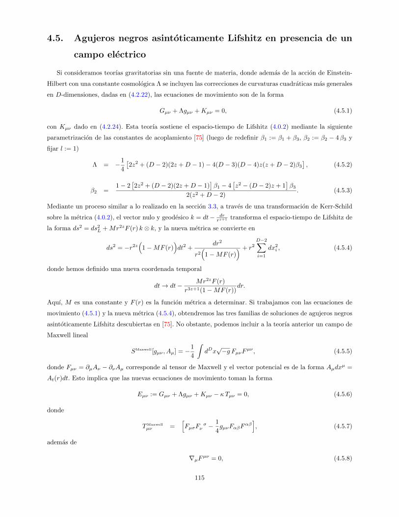
4.5. Agujeros negros asintoticamente Lifshitz en presencia de un
campo electrico
Si consideramos teorıas gravitatorias sin una fuente de materia, donde ademas de la accion de Einstein-
Hilbert con una constante cosmologica Λ se incluyen las correcciones de curvaturas cuadraticas mas generales
en D-dimensiones, dadas en (4.2.22), las ecuaciones de movimiento son de la forma
Gµν + Λgµν +Kµν = 0, (4.5.1)
con Kµν dado en (4.2.24). Esta teorıa sostiene el espacio-tiempo de Lifshitz (4.0.2) mediante la siguiente
parametrizacion de las constantes de acoplamiento [75] (luego de redefinir β1 := β1 + β3, β2 := β2 − 4β3 y
fijar l := 1)
Λ = −1
4
[2z2 + (D − 2)(2z +D − 1)− 4(D − 3)(D − 4)z(z +D − 2)β3
], (4.5.2)
β2 =1− 2
[2z2 + (D − 2)(2z +D − 1)
]β1 − 4
[z2 − (D − 2)z + 1
]β3
2(z2 +D − 2). (4.5.3)
Mediante un proceso similar a lo realizado en la seccion 3.3, a traves de una transformacion de Kerr-Schild
sobre la metrica (4.0.2), el vector nulo y geodesico k = dt− drrz+1 transforma el espacio-tiempo de Lifshitz de
la forma ds2 = ds2L +Mr2zF (r) k ⊗ k, y la nueva metrica se convierte en
ds2 = −r2z(
1−MF (r))dt2 +
dr2
r2(
1−MF (r)) + r2
D−2∑
i=1
dx2i , (4.5.4)
donde hemos definido una nueva coordenada temporal
dt→ dt− Mr2zF (r)
r3z+1(1−MF (r))dr.
Aquı, M es una constante y F (r) es la funcion metrica a determinar. Si trabajamos con las ecuaciones de
movimiento (4.5.1) y la nueva metrica (4.5.4), obtendremos las tres familias de soluciones de agujeros negros
asintoticamente Lifshitz descubiertas en [75]. No obstante, podemos incluir a la teorıa anterior un campo de
Maxwell lineal
SMaxwell[gµν , Aµ] = −1
4
∫dDx√−g FµνFµν , (4.5.5)
donde Fµν = ∂µAν − ∂νAµ corresponde al tensor de Maxwell y el vector potencial es de la forma Aµdxµ =
At(r)dt. Esto implica que las nuevas ecuaciones de movimiento toman la forma
Eµν := Gµν + Λgµν +Kµν − κTµν = 0, (4.5.6)
donde
TMaxwell
µν =[FµσF
σν −
1
4gµνFαβF
αβ], (4.5.7)
ademas de
∇µFµν = 0, (4.5.8)
115

y κ es una constante de acoplamiento. Asimismo, por medio de la metrica (4.5.4), la ecuacion (4.5.8) se
convierte en
Frt = Qrz−D+1,
donde Q es una constante de integracion.
Desde el punto de vista del formalismo cuasilocal, tenemos que tanto el termino de superficie Θµ como
el potencial de Noether Kµν son dados por
Θµ(δg, δA) = Θµgrav(δg) +
√−g ∂L
∂ (∂µAν)δAν , Kµν = Kµν
grav −√−g ∂L
∂ (∂µAν)ξσAσ, (4.5.9)
donde
∂L
∂ (∂µAν)= −Fµν . (4.5.10)
Por otro lado, los efectos de la transformacion Kerr-Schild conllevan a expandir las ecuaciones de movi-
miento (4.5.6) de la forma
Ett = MΣ1 +M2Σ2 +κQ2
2 r2(D−2)= 0,
Err = M (Σ1 − Σ3) +M2 (Σ2 + FΣ3) +κQ2
2 r2(D−2)= 0,
Eii = M (Σ1 − Σ4) +M2(
Σ5 − F (Σ1 − Σ4))− κQ2
2 r2(D−2)= 0, (4.5.11)
donde por simplicidad hemos definido
Σ1 =
4∑
i=0
σ1i ri d
iF
dri, Σ2 = F
(4∑
i=0
σ2i ri d
iF
dri
)+ rF ′
(3∑
i=1
ψ2i ri d
iF
dri
)+ ω22 r
4 (F ′′)2,
Σ3 =
4∑
i=0
σ3i ri d
iF
dri, Σ4 =
4∑
i=0
σ4i ri d
iF
dri, (4.5.12)
Σ5 = F(σ50 F + σ52 r
2 F ′′)
+ rF ′(
3∑
i=0
ψ5i ri d
iF
dri
)+ ω52 r
4 (F ′′)2.
Para ser lo mas claro posible, los diferentes coeficientes σij , ψij y ωij son proporcionados en el Apendice.
De las dos primeras ecuaciones de (4.5.11) se tiene que Σ3 = 0. Esto ultimo corresponde a una ecuacion
diferencial de Cauchy de cuarto orden para la funcion metrica F (r), cuya solucion se puede expresar como
F (r) =
4∑
i=1
Cirαi
, (4.5.13)
donde los Ci’s son constantes de integracion, mientras que los αi’s son raıces del polinomio caracterıstico
σ34α4i + (−σ33 + 6σ34)α3
i + (σ32 − 3σ33 + 11σ34)α2i + (−σ31 + σ32 − 2σ33 + 6σ34)αi + σ30 = 0.
Adicionalmente, por medio de la combinacion Ett +Eii = 0 y la ecuacion Ett = 0, nos permiten concluir que
solamente una de las constantes Ci es no nula y podemos mostrar la existencia de cuatro interesantes familias
de agujeros negros cargados asintoticamente Lifshitz en dimension D arbitraria, las cuales estudiaremos a
continuacion y corresponden a los resultados presentes en el artıculo [4].
116
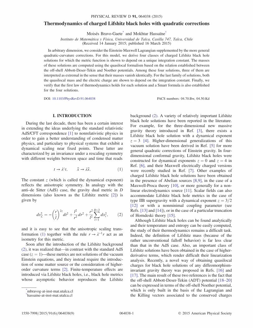
Thermodynamics of charged Lifshitz black holes with quadratic corrections
Moisés Bravo-Gaete* and Mokhtar Hassaïne†
Instituto de Matemática y Física, Universidad de Talca, Casilla 747, Talca, Chile(Received 14 January 2015; published 16 March 2015)
In arbitrary dimension, we consider the Einstein-Maxwell Lagrangian supplemented by the more generalquadratic-curvature corrections. For this model, we derive four classes of charged Lifshitz black holesolutions for which the metric function is shown to depend on a unique integration constant. The massesof these solutions are computed using the quasilocal formalism based on the relation established betweenthe off-shell Abbott-Deser-Tekin and Noether potentials. Among these four solutions, three of them areinterpreted as extremal in the sense that their masses vanish identically. For the last family of solutions, boththe quasilocal mass and the electric charge are shown to depend on the integration constant. Finally, weverify that the first law of thermodynamics holds for each solution and a Smarr formula is also establishedfor the four solutions.
DOI: 10.1103/PhysRevD.91.064038 PACS numbers: 04.70.Bw, 04.50.Kd
I. INTRODUCTION
During the last decade, there has been a certain interestin extending the ideas underlying the standard relativisticAdS/CFT correspondence [1] to nonrelativistic physics inorder to gain a better understanding of condensed matterphysics, and particulary to physical systems that exhibit adynamical scaling near fixed points. These latter arecharacterized by an invariance under a rescaling symmetrywith different weights between space and time that reads
t → λzt; ~x → λ~x: ð1Þ
The constant z (which is called the dynamical exponent)reflects the anisotropic symmetry. In analogy with theanti–de Sitter (AdS) case, the gravity dual metric in Ddimensions (also known as the Lifshitz metric [2]) isgiven by
ds2L ¼ −rl
2zdt2 þ l2
r2dr2 þ r2
l2XD−2
i¼1
dx2i ; ð2Þ
and it is easy to see that the anisotropic scaling trans-formation (1) together with the rule r → λ−1r act as anisometry for this metric.Soon after the introduction of the Lifshitz background
(2), it was realized that—in contrast with the standard AdScase (z ¼ 1)—these metrics are not solutions of the vacuumEinstein equations, and they instead require the introduc-tion of some matter source or the consideration of higher-order curvature terms [2]. Finite-temperature effects areintroduced via Lifshitz black holes, i.e., black hole metricswhose asymptotic behavior reproduces the Lifshitz
background (2). A variety of relatively important Lifshitzblack hole solutions have been reported in the literature.For example, for the three-dimensional new massivegravity theory introduced in Ref. [3], there exists aLifshitz black hole solution with a dynamical exponentz ¼ 3 [4]. Higher-dimensional generalizations of thisvacuum solution have been derived in Ref. [5] for moregeneral quadratic corrections of Einstein gravity. In four-dimensional conformal gravity, Lifshitz black holes wereconstructed for dynamical exponents z ¼ 0 and z ¼ 4 inRef. [6], and their Maxwell electrically charged versionswere recently studied in Ref. [7]. Other examples ofcharged Lifshitz black hole solutions have been obtainedin the presence of Abelian sources [8,9], in the case of aMaxwell-Proca theory [10], or more generally for a non-linear electrodynamics source [11]. Scalar fields can alsoaccommodate Lifshitz black hole metrics in the case oftype IIB supergravity with a dynamical exponent z ¼ 3=2[12] or with a nonminimal coupling parameter (seeRefs. [13] and [14]), or in the case of a particular truncationof Horndeski theory [15].Although Lifshitz black holes can be found analytically
and their temperature and entropy can be easily computed,the study of their thermodynamics remains a difficult task.Indeed, the definition of Lifshitz mass (because of therather unconventional falloff behavior) is far less clearthan that in the AdS case. Also, an important class ofLifshitz solutions have been obtained in the case of higher-derivative terms, which render difficult their linearizationanalysis. Recently, a novel way of obtaining quasilocalcharges for black hole solutions of any diffeomorphism-invariant gravity theory was proposed in Refs. [16] and[17]. The main result of these two references is the fact thatthe off-shell Abbott-Deser-Tekin (ADT) potential [18–20]can be expressed in terms of the off-shell Noether potential,which is only built in the basis of the Lagrangian andthe Killing vectors associated to the conserved charges
*mbravog‑at‑inst‑mat.utalca.cl†hassaine‑at‑inst‑mat.utalca.cl
PHYSICAL REVIEW D 91, 064038 (2015)
1550-7998=2015=91(6)=064038(9) 064038-1 © 2015 American Physical Society

(without having to consider the linearization of the fieldequations). Another important feature of this method lies inthe fact that it may apply for arbitrary asymptotic space-times, and not necessarily for asymptotically flat or AdSspacetimes. For example, this formalism has been shownto be effective in obtaining the correct mass of the z ¼ 3Lifshitz black hole solution of new massive gravity [4] (seealso Ref. [17]). More recently, the authors of Ref. [14] haveconsidered a model of new massive gravity in threedimensions with a nonminimal scalar field for which theyobtained three classes of Lifshitz black hole solutions. Themasses of these solutions computed within the quasilocalformalism fit perfectly with the first law of thermodynam-ics, and as an additional check they showed that theseexpressions for the masses are in accordance with theanisotropic Cardy formula [21] assuming that the groundstate is the respective soliton [14].In the present paper, we further explore this quasilocal
formalism in the case of charged Lifshitz black holes. Inarbitrary dimensions D, we consider the Einstein-MaxwellLagrangian supplemented by a cosmological constant withthe quadratic corrections built from the scalar curvature R,the Ricci tensor Rμν, and the Riemann tensor Rμνρσ as
S ¼ 1
2κ
ZdDx
ffiffiffiffiffiffi−g
p ðR − 2Λþ β1R2 þ β2RαβRαβ
þ β3RαβμνRαβμνÞ − 1
4
ZdDx
ffiffiffiffiffiffi−g
pFαβFαβ
¼Z
dDxffiffiffiffiffiffi−g
pL; ð3Þ
where Fαβ ¼ ∂αAβ − ∂βAα corresponds to the field strengthof the Maxwell field, and the βi are constants. The fieldequations obtained by varying the action (3) read
Eμν ≔ Gμν þ Λgμν þ Kμν − κTμν ¼ 0; ð4aÞ
∇μFμν ¼ 0; ð4bÞ
where
Tμν ¼ FμσFσν −
1
4gμνFαβFαβ; ð4cÞ
Kμν ¼ ðβ2 þ 4β3ÞRμν þ1
2ð4β1 þ β2ÞgμνR
− ð2β1 þ β2 þ 2β3Þ∇μ∇νRþ 2β3RμγαβRνγαβ
þ 2ðβ2 þ 2β3ÞRμανβRαβ − 4β3RμαRνα þ 2β1RRμν
−1
2ðβ1R2 þ β2RαβRαβ þ β3RαβγδRαβγδÞgμν: ð4dÞ
We are interested in looking for charged black holesolutions of the field equations (4) with a purely electricansatz, such that asymptotically the metric behaves like the
Lifshitz spacetime (2). In doing so, we opt for the followingLifshitz-type ansatz:
ds2D ¼ −rl
2zfðrÞdt2 þ l2
r2dr2
fðrÞ þr2
l2XD−2
i¼1
dx2i ; ð5Þ
where we require the unknown metric function fðrÞ tosatisfy limr→þ∞fðrÞ ¼ 1, and the Maxwell potential to beof the form Aμdxμ ¼ AtðrÞdt.The paper is organized as follows. In the next section, we
show that the metric function within our ansatz (5) behavesgenerically as fðrÞ ¼ 1 −MðlrÞχ , whereM is an integrationconstant and χ is a positive constant that always dependson the dimension D. Using this result together with theintegration of the Maxwell equation (4b), we write downthe generic formula for the quasilocal mass associatedto the Killing vector ξμ∂μ ¼ ∂t. In Sec. III, we exhibitexplicitly the four families of charged Lifshitz black holesolutions, and for each of them we compute the mass, theelectric charge, and the entropy, and we verify that the firstlaw of thermodynamics holds in each case. In Sec. IV wediscuss the lower-dimensional cases (D ¼ 3 and D ¼ 4),and in the last section we report our conclusions. Finally, anappendix is added for clarity, where we give some of theformulas needed to derive our results.
II. QUASILOCAL MASS, ENTROPY,AND ELECTRIC CHARGE
In this section, wewill show that themetric functionwithinour ansatz (5) behaves generically as fðrÞ¼1−MðlrÞχ , andwith this result [together with the integration of the Maxwellequation (4b)]wewill express in a genericway the expressionof the quasilocal mass. The details concerning the explicitsolutions will be given in the next section.Considering the metric ansatz (5), the following combi-
nation of the Einstein equations [Eq. (4a)] yields a fourth-order Cauchy differential equation for the unknown metricfunction fðrÞ [which is given by Eq. (A1) in the Appendix]:
−l4
fðrÞ ðEtt − Er
rÞ ¼ 0: ð6Þ
The solution of fðrÞ is generically expressed as
fðrÞ ¼ 1 −X4i¼1
Mi
lr
αi; ð7Þ
where the Mi are some integration constants and the αi arethe roots of the characteristic polynomial. Before followingthis generic analysis, we would like to stress two things.First, there also exists the possibility of having multipleroots for which the metric function fðrÞ will involvelogarithmic contributions, but in these cases the remaining
MOISÉS BRAVO-GAETE AND MOKHTAR HASSA PHYSICAL REVIEW D 91, 064038 (2015)
064038-2
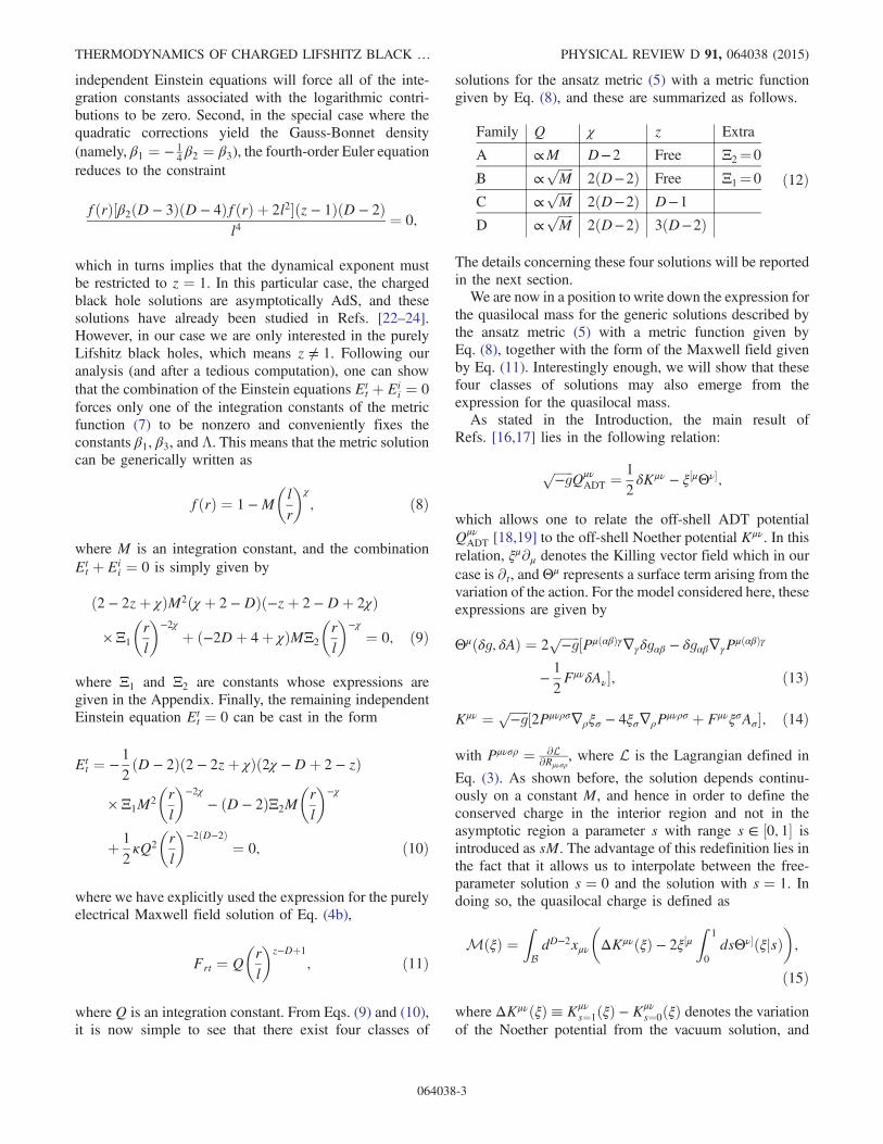
independent Einstein equations will force all of the inte-gration constants associated with the logarithmic contri-butions to be zero. Second, in the special case where thequadratic corrections yield the Gauss-Bonnet density(namely, β1 ¼ − 1
4β2 ¼ β3), the fourth-order Euler equation
reduces to the constraint
fðrÞ½β2ðD − 3ÞðD − 4ÞfðrÞ þ 2l2ðz − 1ÞðD − 2Þl4
¼ 0;
which in turns implies that the dynamical exponent mustbe restricted to z ¼ 1. In this particular case, the chargedblack hole solutions are asymptotically AdS, and thesesolutions have already been studied in Refs. [22–24].However, in our case we are only interested in the purelyLifshitz black holes, which means z ≠ 1. Following ouranalysis (and after a tedious computation), one can showthat the combination of the Einstein equations Et
t þ Eii ¼ 0
forces only one of the integration constants of the metricfunction (7) to be nonzero and conveniently fixes theconstants β1, β3, and Λ. This means that the metric solutioncan be generically written as
fðrÞ ¼ 1 −M
lr
χ
; ð8Þ
where M is an integration constant, and the combinationEtt þ Ei
i ¼ 0 is simply given by
ð2 − 2zþ χÞM2ðχ þ 2 −DÞð−zþ 2 −Dþ 2χÞ
× Ξ1
rl
−2χ
þ ð−2Dþ 4þ χÞMΞ2
rl
−χ
¼ 0; ð9Þ
where Ξ1 and Ξ2 are constants whose expressions aregiven in the Appendix. Finally, the remaining independentEinstein equation Et
t ¼ 0 can be cast in the form
Ett ¼ −
1
2ðD − 2Þð2 − 2zþ χÞð2χ −Dþ 2 − zÞ
× Ξ1M2
rl
−2χ
− ðD − 2ÞΞ2M
rl
−χ
þ 1
2κQ2
rl
−2ðD−2Þ
¼ 0; ð10Þ
where we have explicitly used the expression for the purelyelectrical Maxwell field solution of Eq. (4b),
Frt ¼ Q
rl
z−Dþ1
; ð11Þ
where Q is an integration constant. From Eqs. (9) and (10),it is now simple to see that there exist four classes of
solutions for the ansatz metric (5) with a metric functiongiven by Eq. (8), and these are summarized as follows.
Family Q χ z Extra
A ∝M D−2 Free Ξ2¼0
B ∝ffiffiffiffiffiM
p2ðD−2Þ Free Ξ1¼0
C ∝ffiffiffiffiffiM
p2ðD−2Þ D−1
D ∝ffiffiffiffiffiM
p2ðD−2Þ 3ðD−2Þ
ð12Þ
The details concerning these four solutions will be reportedin the next section.We are now in a position to write down the expression for
the quasilocal mass for the generic solutions described bythe ansatz metric (5) with a metric function given byEq. (8), together with the form of the Maxwell field givenby Eq. (11). Interestingly enough, we will show that thesefour classes of solutions may also emerge from theexpression for the quasilocal mass.As stated in the Introduction, the main result of
Refs. [16,17] lies in the following relation:
ffiffiffiffiffiffi−g
pQμν
ADT ¼ 1
2δKμν − ξ½μΘν;
which allows one to relate the off-shell ADT potentialQμν
ADT [18,19] to the off-shell Noether potential Kμν. In thisrelation, ξμ∂μ denotes the Killing vector field which in ourcase is ∂t, and Θμ represents a surface term arising from thevariation of the action. For the model considered here, theseexpressions are given by
Θμðδg; δAÞ ¼ 2ffiffiffiffiffiffi−g
p ½PμðαβÞγ∇γδgαβ − δgαβ∇γPμðαβÞγ
−1
2FμνδAν; ð13Þ
Kμν ¼ ffiffiffiffiffiffi−g
p ½2Pμνρσ∇ρξσ − 4ξσ∇ρPμνρσ þ FμνξσAσ; ð14Þ
with Pμνσρ ¼ ∂L∂Rμνσρ
, where L is the Lagrangian defined in
Eq. (3). As shown before, the solution depends continu-ously on a constant M, and hence in order to define theconserved charge in the interior region and not in theasymptotic region a parameter s with range s ∈ ½0; 1 isintroduced as sM. The advantage of this redefinition lies inthe fact that it allows us to interpolate between the free-parameter solution s ¼ 0 and the solution with s ¼ 1. Indoing so, the quasilocal charge is defined as
MðξÞ ¼ZBdD−2xμν
ΔKμνðξÞ − 2ξ½μ
Z1
0
dsΘνðξjsÞ;
ð15Þ
where ΔKμνðξÞ≡ Kμνs¼1ðξÞ − Kμν
s¼0ðξÞ denotes the variationof the Noether potential from the vacuum solution, and
THERMODYNAMICS OF CHARGED LIFSHITZ BLACK … PHYSICAL REVIEW D 91, 064038 (2015)
064038-3
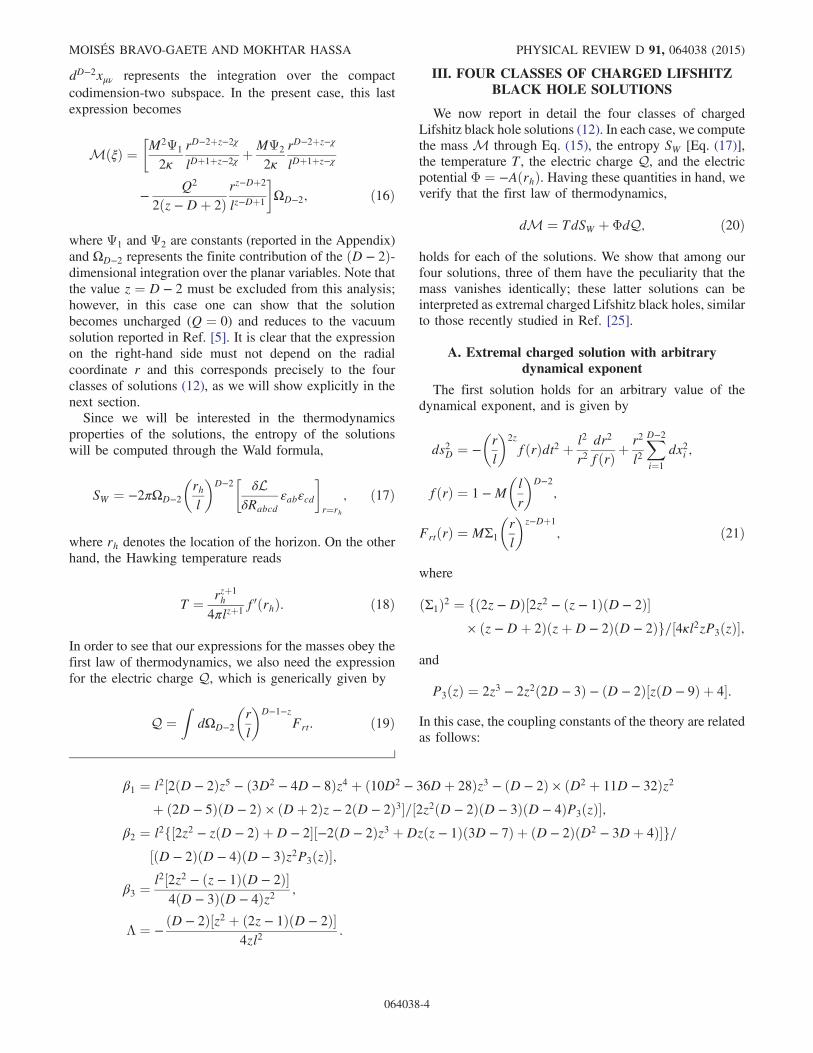
dD−2xμν represents the integration over the compactcodimension-two subspace. In the present case, this lastexpression becomes
MðξÞ ¼M2Ψ1
2κ
rD−2þz−2χ
lDþ1þz−2χ þMΨ2
2κ
rD−2þz−χ
lDþ1þz−χ
−Q2
2ðz −Dþ 2Þrz−Dþ2
lz−Dþ1
ΩD−2; ð16Þ
where Ψ1 and Ψ2 are constants (reported in the Appendix)and ΩD−2 represents the finite contribution of the ðD − 2Þ-dimensional integration over the planar variables. Note thatthe value z ¼ D − 2 must be excluded from this analysis;however, in this case one can show that the solutionbecomes uncharged (Q ¼ 0) and reduces to the vacuumsolution reported in Ref. [5]. It is clear that the expressionon the right-hand side must not depend on the radialcoordinate r and this corresponds precisely to the fourclasses of solutions (12), as we will show explicitly in thenext section.Since we will be interested in the thermodynamics
properties of the solutions, the entropy of the solutionswill be computed through the Wald formula,
SW ¼ −2πΩD−2
rhl
D−2
δL
δRabcdεabεcd
r¼rh
; ð17Þ
where rh denotes the location of the horizon. On the otherhand, the Hawking temperature reads
T ¼ rzþ1h
4πlzþ1f0ðrhÞ: ð18Þ
In order to see that our expressions for the masses obey thefirst law of thermodynamics, we also need the expressionfor the electric charge Q, which is generically given by
Q ¼Z
dΩD−2
rl
D−1−z
Frt: ð19Þ
III. FOUR CLASSES OF CHARGED LIFSHITZBLACK HOLE SOLUTIONS
We now report in detail the four classes of chargedLifshitz black hole solutions (12). In each case, we computethe mass M through Eq. (15), the entropy SW [Eq. (17)],the temperature T, the electric charge Q, and the electricpotential Φ ¼ −AðrhÞ. Having these quantities in hand, weverify that the first law of thermodynamics,
dM ¼ TdSW þ ΦdQ; ð20Þ
holds for each of the solutions. We show that among ourfour solutions, three of them have the peculiarity that themass vanishes identically; these latter solutions can beinterpreted as extremal charged Lifshitz black holes, similarto those recently studied in Ref. [25].
A. Extremal charged solution with arbitrarydynamical exponent
The first solution holds for an arbitrary value of thedynamical exponent, and is given by
ds2D ¼ −rl
2zfðrÞdt2 þ l2
r2dr2
fðrÞ þr2
l2XD−2
i¼1
dx2i ;
fðrÞ ¼ 1 −M
lr
D−2
;
FrtðrÞ ¼ MΣ1
rl
z−Dþ1
; ð21Þ
where
ðΣ1Þ2 ¼ fð2z −DÞ½2z2 − ðz − 1ÞðD − 2Þ× ðz −Dþ 2ÞðzþD − 2ÞðD − 2Þg=½4κl2zP3ðzÞ;
and
P3ðzÞ ¼ 2z3 − 2z2ð2D − 3Þ − ðD − 2Þ½zðD − 9Þ þ 4:In this case, the coupling constants of the theory are relatedas follows:
β1 ¼ l2½2ðD − 2Þz5 − ð3D2 − 4D − 8Þz4 þ ð10D2 − 36Dþ 28Þz3 − ðD − 2Þ × ðD2 þ 11D − 32Þz2þ ð2D − 5ÞðD − 2Þ × ðDþ 2Þz − 2ðD − 2Þ3=½2z2ðD − 2ÞðD − 3ÞðD − 4ÞP3ðzÞ;
β2 ¼ l2f½2z2 − zðD − 2Þ þD − 2½−2ðD − 2Þz3 þDzðz − 1Þð3D − 7Þ þ ðD − 2ÞðD2 − 3Dþ 4Þg=½ðD − 2ÞðD − 4ÞðD − 3Þz2P3ðzÞ;
β3 ¼l2½2z2 − ðz − 1ÞðD − 2Þ
4ðD − 3ÞðD − 4Þz2 ;
Λ ¼ −ðD − 2Þ½z2 þ ð2z − 1ÞðD − 2Þ
4zl2:
MOISÉS BRAVO-GAETE AND MOKHTAR HASSA PHYSICAL REVIEW D 91, 064038 (2015)
064038-4

Plugging this solution into Eq. (16) implies that themass M vanishes identically. On the other hand, the Waldentropy is nonzero and given by
SW ¼ 4πΩD−2ðΣ1Þ2rD−2h
ðz −Dþ 2ÞðD − 2ÞlD−4 ; ð22Þ
while the Hawking temperature is
T ¼ ðD − 2Þrzh4πlzþ1
: ð23Þ
The charge and the electric potential read, respectively,
Q ¼ Σ1ΩD−2
rhl
D−2
; ð24Þ
and
Φ ¼ −AðrhÞ ¼ −Σ1r
zh
ðz −Dþ 2Þlz−1 : ð25Þ
It is straightforward to check that in spite of having zeromass, the first law (20) still holds in the form
dM ¼ 0 ¼ TdSW þ ΦdQ;
and hence this solution can be interpreted as an extremalcharged Lifshitz black hole.
B. Second extremal family with an arbitrary z
A second extremal family of solutions is found whenχ ¼ 2ðD − 2Þ and for an arbitrary value of the dynamicalexponent,
ds2D ¼ −rl
2zfðrÞdt2 þ l2
r2dr2
fðrÞ þr2
l2XD−2
i¼1
dx2i ;
fðrÞ ¼ 1 −M
lr
2ðD−2Þ
;
Frt ¼ffiffiffiffiffiM
pΣ2
rl
z−Dþ1
; ð26Þ
where
ðΣ2Þ2 ¼ f½2z2 þ ðD− 2ÞðD− 1− 4zÞ× ðD− 2Þðzþ 2D− 4Þðz−Dþ 2Þg=½2κl2zP2ðzÞ;
with
P2ðzÞ ¼ z2 − ðD − 2ÞðD − 4þ 2zÞ:The space of parameters is defined by
β1 ¼ l2½2ðD − 2Þz4 þ ð25D − 7D2 − 20Þz3 þ 2ðD − 2Þð3D2 − 8Dþ 3Þz2 − ðD − 2Þ× ð3D2 − 5D − 4Þz − 2ðD − 4ÞðD − 2Þ3=½4ðD − 2ÞzðD − 3ÞðD − 4Þðz −Dþ 2ÞP2ðzÞ;
β2 ¼ l2f½−4ðD − 2Þz2 þ ð20 − 25Dþ 7D2Þzþ 2ðD − 1ÞðD − 2ÞðD − 4Þ× ½2z2 þ ðD − 2ÞðD − 1 − 4zÞg=½4ðD − 4Þzðz −Dþ 2ÞðD − 3ÞðD − 2ÞP2ðzÞ;
β3 ¼l2½2z2 þ ðD − 2ÞðD − 4z − 1Þ4ðD − 3ÞðD − 4Þðz −Dþ 2Þz ;
Λ ¼ ðD − 2Þ½−z2 þ ðD − 2ÞðD − 1 − zÞ2l2ðz −Dþ 2Þ :
Note that this solution has been recently reported inRef. [7]. As before, the mass vanishes, while the otherrelevant thermodynamical quantities are given by
SW ¼ 2πΩD−2ðΣ2Þ2rD−2h
ðD − 2Þðz −Dþ 2ÞlD−4 ; ð27aÞ
T ¼ ðD − 2Þrzh2πlzþ1
; ð27bÞ
Q ¼ Σ2ΩD−2
rhl
D−2
; ð27cÞ
Φ ¼ −Σ2r
zh
ðz −Dþ 2Þlz−1 ; ð27dÞ
in accordance with the results obtained in Ref. [7] viathe Wald formalism. The extremal character of thecharged solution is encoded in the relation dM¼0¼TdSWþΦdQ.
C. Third extremal solution with fixed z ¼ ðD − 1ÞA third family of solutions is found when the
dynamical exponent takes the value z ¼ ðD − 1Þ, and isgiven by
THERMODYNAMICS OF CHARGED LIFSHITZ BLACK … PHYSICAL REVIEW D 91, 064038 (2015)
064038-5
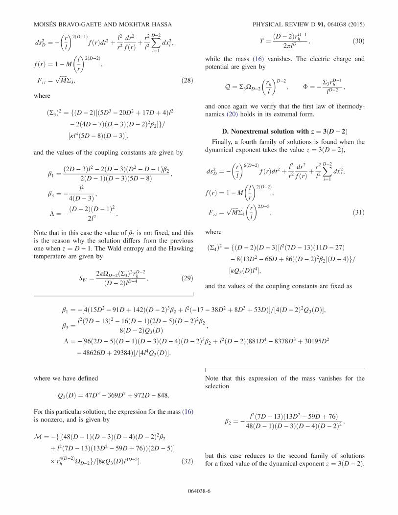
ds2D ¼ −rl
2ðD−1Þ
fðrÞdt2 þ l2
r2dr2
fðrÞ þr2
l2XD−2
i¼1
dx2i ;
fðrÞ ¼ 1 −M
lr
2ðD−2Þ
;
Frt ¼ffiffiffiffiffiM
pΣ3; ð28Þ
where
ðΣ3Þ2 ¼ fðD − 2Þ½ð5D3 − 20D2 þ 17Dþ 4Þl2− 2ð4D − 7ÞðD − 3ÞðD − 2Þ2β2g=½κl4ð5D − 8ÞðD − 3Þ;
and the values of the coupling constants are given by
β1 ¼ð2D − 3Þl2 − 2ðD − 3ÞðD2 −D − 1Þβ2
2ðD − 1ÞðD − 3Þð5D − 8Þ ;
β3 ¼ −l2
4ðD − 3Þ ;
Λ ¼ −ðD − 2ÞðD − 1Þ2
2l2:
Note that in this case the value of β2 is not fixed, and thisis the reason why the solution differs from the previousone when z ¼ D − 1. The Wald entropy and the Hawkingtemperature are given by
SW ¼ 2πΩD−2ðΣ3Þ2rD−2h
ðD − 2ÞlD−4 ; ð29Þ
T ¼ ðD − 2ÞrD−1h
2πlD; ð30Þ
while the mass (16) vanishes. The electric charge andpotential are given by
Q ¼ Σ3ΩD−2
rhl
D−2
; Φ ¼ −Σ3rD−1
h
lD−2 ;
and once again we verify that the first law of thermody-namics (20) holds in its extremal form.
D. Nonextremal solution with z ¼ 3ðD − 2ÞFinally, a fourth family of solutions is found when the
dynamical exponent takes the value z ¼ 3ðD − 2Þ,
ds2D ¼ −rl
6ðD−2Þ
fðrÞdt2 þ l2
r2dr2
fðrÞ þr2
l2XD−2
i¼1
dx2i ;
fðrÞ ¼ 1 −Mlr
2ðD−2Þ
;
Frt ¼ffiffiffiffiffiM
pΣ4
rl
2D−5
; ð31Þ
where
ðΣ4Þ2 ¼ fðD − 2ÞðD − 3Þ½l2ð7D − 13Þð11D − 27Þ− 8ð13D2 − 66Dþ 86ÞðD − 2Þ2β2ðD − 4Þg=½κQ3ðDÞl4;
and the values of the coupling constants are fixed as
β1 ¼ −½4ð15D2 − 91Dþ 142ÞðD − 2Þ3β2 þ l2ð−17 − 38D2 þ 8D3 þ 53DÞ=½4ðD − 2Þ2Q3ðDÞ;
β3 ¼l2ð7D − 13Þ2 − 16ðD − 1Þð2D − 5ÞðD − 2Þ2β2
8ðD − 2ÞQ3ðDÞ ;
Λ ¼ −½96ð2D − 5ÞðD − 1ÞðD − 3ÞðD − 4ÞðD − 2Þ3β2 þ l2ðD − 2Þð881D4 − 8378D3 þ 30195D2
− 48626Dþ 29384Þ=½4l4Q3ðDÞ;
where we have defined
Q3ðDÞ ¼ 47D3 − 369D2 þ 972D − 848:
For this particular solution, the expression for the mass (16)is nonzero, and is given by
M ¼ −f½ð48ðD − 1ÞðD − 3ÞðD − 4ÞðD − 2Þ2β2þ l2ð7D − 13Þð13D2 − 59Dþ 76ÞÞð2D − 5Þ× r4ðD−2Þ
h ΩD−2g=½8κQ3ðDÞl4D−5: ð32Þ
Note that this expression of the mass vanishes for theselection
β2 ¼ −l2ð7D − 13Þð13D2 − 59Dþ 76Þ
48ðD − 1ÞðD − 3ÞðD − 4ÞðD − 2Þ2 ;
but this case reduces to the second family of solutionsfor a fixed value of the dynamical exponent z ¼ 3ðD − 2Þ.
MOISÉS BRAVO-GAETE AND MOKHTAR HASSA PHYSICAL REVIEW D 91, 064038 (2015)
064038-6
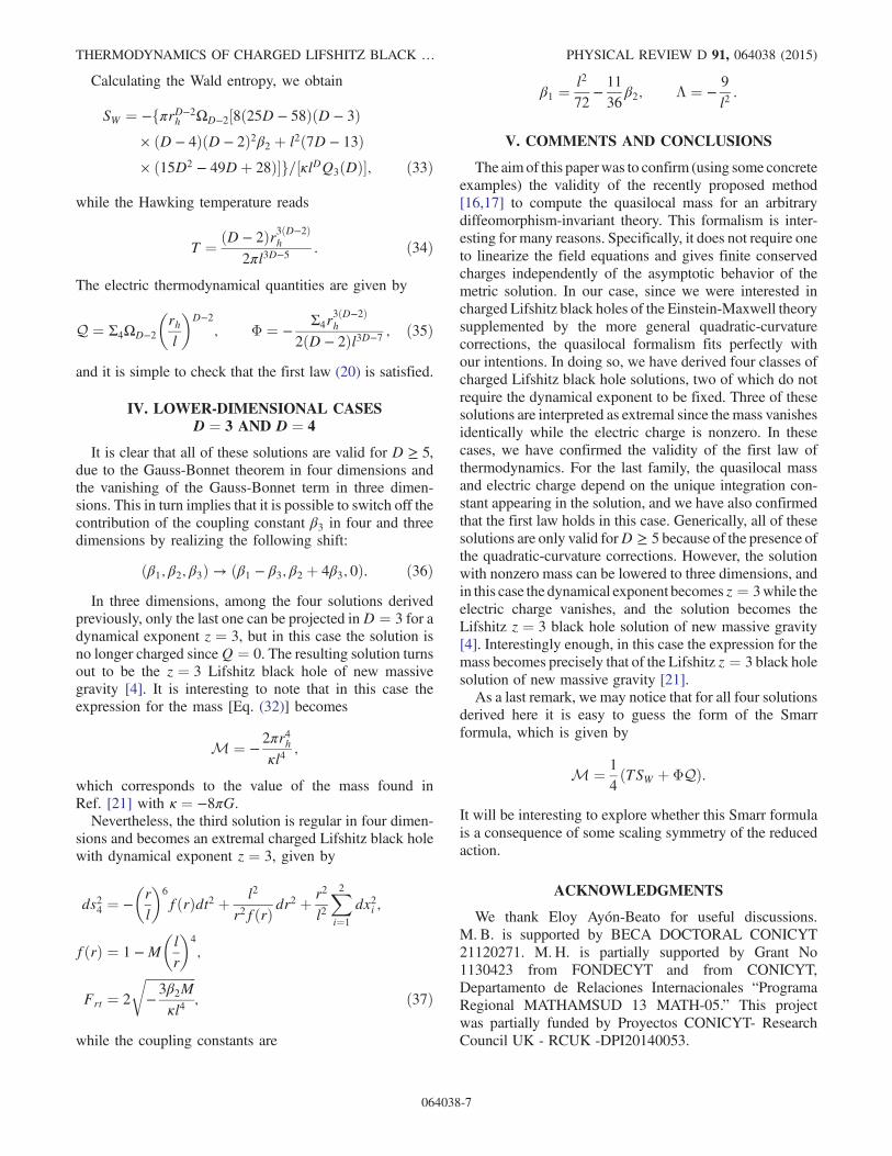
Calculating the Wald entropy, we obtain
SW ¼ −fπrD−2h ΩD−2½8ð25D − 58ÞðD − 3Þ
× ðD − 4ÞðD − 2Þ2β2 þ l2ð7D − 13Þ× ð15D2 − 49Dþ 28Þg=½κlDQ3ðDÞ; ð33Þ
while the Hawking temperature reads
T ¼ ðD − 2Þr3ðD−2Þh
2πl3D−5 : ð34Þ
The electric thermodynamical quantities are given by
Q ¼ Σ4ΩD−2
rhl
D−2
; Φ ¼ −Σ4r
3ðD−2Þh
2ðD − 2Þl3D−7 ; ð35Þ
and it is simple to check that the first law (20) is satisfied.
IV. LOWER-DIMENSIONAL CASESD ¼ 3 AND D ¼ 4
It is clear that all of these solutions are valid for D ≥ 5,due to the Gauss-Bonnet theorem in four dimensions andthe vanishing of the Gauss-Bonnet term in three dimen-sions. This in turn implies that it is possible to switch off thecontribution of the coupling constant β3 in four and threedimensions by realizing the following shift:
ðβ1; β2; β3Þ → ðβ1 − β3; β2 þ 4β3; 0Þ: ð36ÞIn three dimensions, among the four solutions derived
previously, only the last one can be projected inD ¼ 3 for adynamical exponent z ¼ 3, but in this case the solution isno longer charged sinceQ ¼ 0. The resulting solution turnsout to be the z ¼ 3 Lifshitz black hole of new massivegravity [4]. It is interesting to note that in this case theexpression for the mass [Eq. (32)] becomes
M ¼ −2πr4hκl4
;
which corresponds to the value of the mass found inRef. [21] with κ ¼ −8πG.Nevertheless, the third solution is regular in four dimen-
sions and becomes an extremal charged Lifshitz black holewith dynamical exponent z ¼ 3, given by
ds24 ¼ −rl
6
fðrÞdt2 þ l2
r2fðrÞ dr2 þ r2
l2X2i¼1
dx2i ;
fðrÞ ¼ 1 −M
lr
4
;
Frt ¼ 2
ffiffiffiffiffiffiffiffiffiffiffiffiffiffiffiffi−3β2Mκl4
r; ð37Þ
while the coupling constants are
β1 ¼l2
72−11
36β2; Λ ¼ −
9
l2:
V. COMMENTS AND CONCLUSIONS
The aimof this paperwas to confirm (using some concreteexamples) the validity of the recently proposed method[16,17] to compute the quasilocal mass for an arbitrarydiffeomorphism-invariant theory. This formalism is inter-esting for many reasons. Specifically, it does not require oneto linearize the field equations and gives finite conservedcharges independently of the asymptotic behavior of themetric solution. In our case, since we were interested incharged Lifshitz black holes of the Einstein-Maxwell theorysupplemented by the more general quadratic-curvaturecorrections, the quasilocal formalism fits perfectly withour intentions. In doing so, we have derived four classes ofcharged Lifshitz black hole solutions, two of which do notrequire the dynamical exponent to be fixed. Three of thesesolutions are interpreted as extremal since the mass vanishesidentically while the electric charge is nonzero. In thesecases, we have confirmed the validity of the first law ofthermodynamics. For the last family, the quasilocal massand electric charge depend on the unique integration con-stant appearing in the solution, and we have also confirmedthat the first law holds in this case. Generically, all of thesesolutions are only valid forD ≥ 5 because of the presence ofthe quadratic-curvature corrections. However, the solutionwith nonzero mass can be lowered to three dimensions, andin this case the dynamical exponent becomes z ¼ 3while theelectric charge vanishes, and the solution becomes theLifshitz z ¼ 3 black hole solution of new massive gravity[4]. Interestingly enough, in this case the expression for themass becomes precisely that of the Lifshitz z ¼ 3 black holesolution of new massive gravity [21].As a last remark, we may notice that for all four solutions
derived here it is easy to guess the form of the Smarrformula, which is given by
M ¼ 1
4ðTSW þ ΦQÞ:
It will be interesting to explore whether this Smarr formulais a consequence of some scaling symmetry of the reducedaction.
ACKNOWLEDGMENTS
We thank Eloy Ayón-Beato for useful discussions.M. B. is supported by BECA DOCTORAL CONICYT21120271. M. H. is partially supported by Grant No1130423 from FONDECYT and from CONICYT,Departamento de Relaciones Internacionales “ProgramaRegional MATHAMSUD 13 MATH-05.” This projectwas partially funded by Proyectos CONICYT- ResearchCouncil UK - RCUK -DPI20140053.
THERMODYNAMICS OF CHARGED LIFSHITZ BLACK … PHYSICAL REVIEW D 91, 064038 (2015)
064038-7
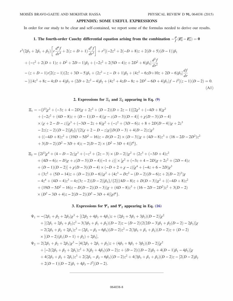
APPENDIX: SOME USEFUL EXPRESSIONS
In order for our study to be clear and self-contained, we report some of the formulas needed to derive our results.
1. The fourth-order Cauchy differential equation arising from the combination − l4f ðEt
t − ErrÞ ¼ 0
r3ð2β3 þ 2β1 þ β2Þrd4fdr4
þ 2ðzþDþ 1Þ d3fdr3
þ r2½ð−2z2 þ 2ð−Dþ 8Þzþ 2ðDþ 5ÞðD − 1ÞÞβ1
þ ð−z2 þ 2ðDþ 1ÞzþD2 þ 2D − 1Þβ2 þ ð−2z2 þ 2ð5D − 4Þzþ 2D2 þ 6Þβ3d2fdr2
− ðzþD − 1Þr½2ðz − 1Þð2zþ 3D − 5Þβ1 þ ð2z2 − z −Dþ 1Þβ2 þ ð4z2 − 6zDþ10zþ 2D − 6Þβ3dfdr
− ½ðð4z2 þ 8z − 4zDþ 4Þβ3 þ ð2Dþ 2z2 − 4Þβ2 þ ð4z2 þ 4zD − 8zþ 2D2 − 6Dþ 4Þβ1Þf − l2ðz − 1ÞðD − 2Þ ¼ 0:
ðA1Þ
2. Expressions for Ξ1 and Ξ2 appearing in Eq. (9)
Ξ1 ¼ −fl2½χ2 þ ð−3zþ 4 − 2DÞχ þ 2z2 þ ðD − 2ÞðDþ 2z − 1Þ½2χ3 þ ð−4Dþ 8Þχ2þ ð−2z2 þ ð4D − 8Þzþ ðD − 1ÞðD − 4ÞÞχ − zðD − 3ÞðD − 4Þ þ χðD − 3ÞðD − 4Þ× ðχ þ 2 −D − zÞ½χ3 þ ð−3D − 2zþ 6Þχ2 þ ð−z2 þ ð3D − 6Þzþ 8þ 2DðD − 4ÞÞχ þ 2z3
− 2zðz − 2ÞðD − 2Þβ2g=f2ðχ þ 2 −D − zÞχ½ðDðD − 3Þ þ 4ðD − 2ÞzÞχ2þ ðð−4Dþ 8Þz2 þ ð19D − 5D2 − 16Þz −DðD − 2Þ × ðD − 3ÞÞχ þ ð4D − 8Þz3 þ ð16 − 2D − 2D2Þz2þ 3ðD − 2ÞðD2 − 3Dþ 4Þz − 2ðD − 2Þ × ðD2 − 3Dþ 4Þl4g;
Ξ2 ¼ f2l2½χ4 þ ð4 −D − 2zÞχ3 þ ð−z2 þ ð2z − 3Þ × ðD − 2ÞÞχ2 þ ð2z3 þ ð−3Dþ 4Þz2þ ð4D − 6Þz −DÞχ þ zðD − 3ÞðD − 4Þð−1þ zÞ × ½χ2 þ ð−3zþ 4 − 2DÞχ þ 2z2 þ ð2D − 4Þzþ ðD − 1ÞðD − 2Þ þ χðD − 3ÞðD − 4Þ × ð−Dþ 2þ χ − zÞ½χ4 þ ð−4zþ 6 − 2DÞχ3þ ð3z2 þ ð5D − 14Þzþ ðD − 2ÞðD − 6ÞÞχ2 þ ð4z3 −Dz2 − ðD − 2ÞðD − 6Þzþ 2ðD − 2Þ2Þχ− 4z4 þ ð4D − 4Þz3 − 4zð3z − 2ÞðD − 2Þβ2g=f2½ðð4D − 8ÞzþDðD − 3ÞÞχ2 þ ðð−4Dþ 8Þz2þ ð19D − 5D2 − 16Þz −DðD − 2ÞðD − 3ÞÞχ þ ð4D − 8Þz3 þ ð16 − 2D − 2D2Þz2 þ 3ðD − 2Þ× ðD2 − 3Dþ 4Þz − 2ðD − 2ÞðD2 − 3Dþ 4Þχl4g:
3. Expressions for Ψ 1 and Ψ 2 appearing in Eq. (16)
Ψ1 ¼ −ð2β1 þ β2 þ 2β3Þχ3 þ ½ð2β2 þ 4β3 þ 4β1Þzþ ð2β2 þ 5β1 þ 3β3ÞðD − 2Þχ2þ ½ð2β1 þ 2β3 þ β2Þz2 − 3ð3β3 þ β1 þ β2ÞðD − 2Þz − ðD − 2Þð2ð2D − 3Þβ1 þ β2ðD − 2Þ − 2β3Þχ− 2ð2β3 þ β2 þ 2β1Þz3 − ð2β1 − β2 − 6β3ÞðD − 2Þz2 − 2ð3β3 þ β1 þ β2ÞðD − 2Þzþ ðD − 2Þ× ½ðD − 2Þðβ1ðD − 1Þ þ β2Þ þ 2β3;
Ψ2 ¼ 2ð2β1 þ β2 þ 2β3Þχ3 − ½4ð2β3 þ 2β1 þ β2Þzþ ð4β3 þ 8β1 þ 3β2ÞðD − 2Þχ2þ ½−2ð2β3 þ β2 þ 2β1Þz2 þ 3ðβ2 þ 4β3ÞðD − 2Þzþ ðD − 2ÞððD − 2Þβ2 þ 4ðD − 1Þβ1 − 4β3Þχþ 4ð2β3 þ β2 þ 2β1Þz3 þ 2ð2β1 − β2 − 6β3ÞðD − 2Þz2 þ 4ð3β3 þ β1 þ β2ÞðD − 2Þz − ½2ðD − 2Þβ2þ 2ðD − 1ÞðD − 2Þβ1 þ 4β3 − l2ðD − 2Þ:
MOISÉS BRAVO-GAETE AND MOKHTAR HASSA PHYSICAL REVIEW D 91, 064038 (2015)
064038-8

[1] J. M. Maldacena, Adv. Theor. Math. Phys. 2, 231 (1998).[2] S. Kachru, X. Liu, and M. Mulligan, Phys. Rev. D 78,
106005 (2008).[3] E. A. Bergshoeff, O. Hohm, and P. K. Townsend, Phys. Rev.
Lett. 102, 201301 (2009).[4] E. Ayon-Beato, A. Garbarz, G. Giribet, and M. Hassaine,
Phys. Rev. D 80, 104029 (2009).[5] E. Ayon-Beato, A. Garbarz, G. Giribet, and M. Hassaine,
J. High Energy Phys. 04 (2010) 030.[6] H. Lu, Y. Pang, C. N. Pope, and J. F. Vazquez-Poritz, Phys.
Rev. D 86, 044011 (2012).[7] Z. Y. Fan and H. Lu, Thermodynamical first laws of black
holes in quadratically extended gravities, arXiv:1501.00006[Phys. Rev. D (to be published)].
[8] M. Taylor, Non-relativistic holography, arXiv:0812.0530.[9] U. Danielsson and L. Thorlacius, J. High Energy Phys. 03
(2009) 070.[10] D.W. Pang, J. High Energy Phys. 01 (2010) 116.[11] A. Alvarez, E. Ayón-Beato, H. A. González, and M.
Hassaïne, J. High Energy Phys. 06 (2014) 041.[12] T. Azeyanagi, W. Li, and T. Takayanagi, J. High Energy
Phys. 06 (2009) 084.[13] F. Correa, M. Hassaine, and J. Oliva, Phys. Rev. D 89,
124005 (2014).
[14] E. Ayon-Beato, M. Bravo-Gaete, F. Correa, M. Hassaine,M.M. Juarez-Aubry, and J. Oliva, First law and anisotropicCardy formula for three-dimensional Lifshitz black holes,arXiv:1501.01244 [Phys. Rev. D (to be published)].
[15] M. Bravo-Gaete and M. Hassaine, Phys. Rev. D 89, 104028(2014).
[16] W. Kim, S. Kulkarni, and S.-H. Yi, Phys. Rev. Lett. 111,081101 (2013).
[17] Y. Gim, W. Kim, and S.-H. Yi, J. High Energy Phys. 07(2014) 002.
[18] S. Deser and B. Tekin, Phys. Rev. Lett. 89, 101101 (2002).[19] S. Deser and B. Tekin, Phys. Rev. D 67, 084009 (2003).[20] C. Senturk, T. C. Sisman, and B. Tekin, Phys. Rev. D 86,
124030 (2012).[21] H. A. Gonzalez, D. Tempo, and R. Troncoso, J. High
Energy Phys. 11 (2011) 066.[22] M. Banados, C. Teitelboim, and J. Zanelli, Phys. Rev. D 49,
975 (1994).[23] J. Crisostomo, R. Troncoso, and J. Zanelli, Phys. Rev. D 62,
084013 (2000).[24] R. Aros, R. Troncoso, and J. Zanelli, Phys. Rev. D 63,
084015 (2001).[25] H. S. Liu and H. Lu, Thermodynamics of Lifshitz black
holes, J. High Energy Phys. 12 (2014) 071.
THERMODYNAMICS OF CHARGED LIFSHITZ BLACK … PHYSICAL REVIEW D 91, 064038 (2015)
064038-9

Capıtulo 5
Teorıa de Horndeski
En la seccion 3.2 estudiamos la gravedad de Lovelock, correspondiente a la extension mas natural de la
Relatividad General para espacio-tiempos de dimensiones superiores. Dado lo anterior, cabe preguntarse si
existen otras teorıas de tal manera que incluyan otros campos no triviales, tales como un campo escalar,
con caracterısticas similares a la teorıa de Lovelock. La respuesta ha sido entregada por G. Horndeski en la
decada de 1970, formulando una teorıa dotada de la metrica gµν , un campo escalar Φ, ası como tambien de
sus derivadas [119] en dimension cuatro, donde se destaca que, aunque el Lagrangiano contiene derivadas de
orden superior, las ecuaciones de movimiento son a lo mas de segundo orden.
Una manera intuitiva de obtener la accion de Horndeski es mediante un modelo de similares caracterısticas
conocido como Galileon [120,121] a traves de la introduccion de cuatro funciones que dependen del termino
cinetico X = − 12gµν∂µΦ∂νΦ y del campo escalar Φ [122], esto es
S[X,Φ, gµν ] =
∫d4x√−g
[K (X,Φ)−G(3) (X,Φ)Φ +G
(4),X
((Φ)
2 − (∇∇Φ)2)
+RG(4)(X,Φ)
− 1
6G
(5),X
((Φ)
3 − 3Φ (∇∇Φ)2
+ 2 (∇∇Φ)3)
+Gµν∇µ∇νΦG(5) (X,Φ)], (5.0.1)
donde hemos definido
G(n),X :=
∂G(n)
∂X, n = 3, 4, 5,
(∇∇Φ)2
:= (∇µ∇νΦ) (∇µ∇νΦ) ,
(∇∇Φ)3
:= (∇µ∇νΦ) (∇µ∇ρΦ) (∇ρ∇νΦ) .
Notemos que para una eleccion de las funciones: K(X,Φ) = X − Λκ , G(4)(X,Φ) = 1
2κ −ξ2Φ2 y G(3) = 0 =
G(5), obtenemos la teorıa asociada a un campo escalar no mınimamente acoplado estudiado en la seccion 3.1
en dimension cuatro, con κ = 8πG . En particular, en este capıtulo estamos interesados en una subclase de
la teorıa (5.0.1) caracterizada por poseer las simetrıas Φ→ −Φ y Φ→ Φ+ constante [123]. Concretamente,
para las expresiones
K(X,Φ) = αX − 2κΛ, G(4)(X,Φ) = κζ +η
2X, G(3) = 0 = G(5),
donde Λ es la constante cosmologica, mientras que κ, ζ, α y η son constantes de acoplamiento, la accion
126
(5.0.1) adquiere la forma
S[gµν ,Φ] =
∫ √−g d4 x
[κ(ζR− 2Λ)− 1
2(αgµν − ηGµν)∇µΦ∇νΦ
]. (5.0.2)
Las ecuaciones de movimiento, respecto a la metrica y al campo escalar, son
ζGµν + Λgµν =1
2κ
[αT (1)
µν + ηT (2)µν
], (5.0.3)
∇µJµ = 0, Jµ = (αgµν − ηGµν)∇νΦ, (5.0.4)
donde los tensores T(i)µν son definidos como
T (1)µν =
(∇µΦ∇νΦ− 1
2gµν∇λΦ∇λΦ
).
T (2)µν =
1
2∇µΦ∇νΦR− 2∇λΦ∇(µΦRλν) −∇λΦ∇ρΦRµλνρ
−(∇µ∇λΦ)(∇ν∇λΦ) + (∇µ∇νΦ)Φ +1
2Gµν(∇Φ)2
−gµν[−1
2(∇λ∇ρΦ)(∇λ∇ρΦ) +
1
2(Φ)2 −∇λΦ∇ρΦRλρ
].
El plan de este capıtulo esta organizado como sigue. En la proxima seccion estudiamos configuraciones de
agujeros negros considerando la accion (5.0.2), donde una de manera de eludir el teorema de no-pelo expuesto
en [124] es imponer que la componente radial de la corriente conservada (5.0.4) se desvanezca trivialmente,
sin la necesidad de aplicar alguna condicion al campo escalar Φ, esto es
αgrr − ηGrr = 0. (5.0.5)
En la seccion 5.2 se dan a conocer las soluciones encontradas en [5], estudiando agujeros negros de Lifshitz,
cuya particularidad esta en la dependencia temporal del campo escalar junto a un valor particular del
exponente dinamico z. Finalmente, en la seccion 5.3 se exponen los resultados presentes en [6], analizando
la termodinamica de agujeros negros, los cuales para el caso tridimensional obtenemos la solucion conocida
como BTZ.
5.1. Agujeros negros en presencia de una fuente particular de la
teorıa de Horndeski
La primera solucion de agujero negro dada la teorıa (5.0.2), sin una constante cosmologica, fue encontrada
en [125], la cual en su notacion tenemos que ζ =m2p
2 , α = 1, κ = 1 y η = zm2p, donde mp es la masa de
Planck y z es un numero real. Considerando un caso particular de la metrica (3.3.1) para un espacio-tiempo
tetradimensional, junto con γ = 1 y un campo escalar de la forma Φ = Φ(r), tenemos que la solucion de este
sistema es de la forma
f(r) =3
4+r2
l2− 2M
m2pr
+
√z
4mprarctan
(mpr√z
), (5.1.1)
g(r) =4(m2
pr2 + z)2f(r)
(m2pr
2 + 2z)2, (5.1.2)
(Φ′(r)
)2= −m
6pr
2(m2pr
2 + 2z)2
4z(m2pr
2 + z)3 f(r), (5.1.3)
127
donde (′) corresponde a la derivada del campo escalar respecto a la coordenada r, M es una constante
de integracion asociada a la masa, mientras que l se define como l2 := 12z/m2p. Esta solucion describe un
agujero negro con un horizonte de eventos localizado en r = rh para M > 0. Adicionalmente, en [125] se
analizaron las propiedades termodinamicas mediante la continuacion analıtica t→ −iτ . En orden de evitar
la singularidad conica en el horizonte de la metrica Euclidiana, el tiempo Euclidiano τ es periodico con
periodo β
β =4π√gττgrr
g′ττ
∣∣∣∣∣r=rh
=8πzrh
(m2pr
2h + 2z)
, (5.1.4)
y la temperatura de Hawking esta dada por T = β−1. De igual manera, para encontrar los otros parametros
termodinamicos, se considero la tecnica de S. W. Hawking y D. N. Page [126], definiendo la accion Euclidiana
regularizada de la forma
SReg := SE(gµν ,Φ)− SE(g(0)µν ,Φ
(0)), (5.1.5)
donde g(0)µν y Φ(0) corresponden a la metrica y al campo escalar considerando M = 0 (los cuales describen
un soliton gravitacional) a la solucion dada por las expresiones (5.1.1 - 5.1.3), mientras que la integral de la
accion esta definida entre el horizonte rh y R rh. Si consideramos la constante β0 como la temperatura
inversa del soliton, esta se relaciona con β requiriendo la condicion
β20f(r = R,M = 0) = β2f(r = R,M), (5.1.6)
para posteriormente tomar el lımite R→ +∞ en la accion regularizada (5.1.5). Lo anterior permite obtener
la masa MReg = ∂SReg/∂β, la entropıa S = βMReg − SReg y el calor especıfico C = ∂MReg/∂T como
MReg = M +mp√z x3(x2 + 2)2
8(x2 − 2)(x2 + 1), (5.1.7)
S =πzx2(2x4 + x2 − 2)
(x2 + 1)(x2 − 2), (5.1.8)
C =2πzx2(x2 + 2)(2x8 − 4x6 − 11x4 − 4x2 + 4)
(x2 + 1)2(x2 − 2)3, (5.1.9)
donde se ha definido x := mprh/√z.
A pesar de esta rica estructura termodinamica, considerando el caso z > 0 tenemos que el cuadrado de
la derivada del campo escalar (5.1.3) es negativo para r > rh, lo cual implica que el campo escalar Φ es
complejo. Sin embargo, en [127] logran eludir este inconveniente extendiendo la teorıa a traves de la inclusion
de una constante cosmologica a la accion, haciendo posible encontrar agujeros negros con un campo escalar
real para la region fuera del horizonte de eventos, primero para dimension cuatro y luego para una extension
dimensional arbitraria. Concretamente, para κ = 116πG , ζ = 1 y un ansatz metrico de la forma (3.3.1), la
solucion para las ecuaciones de movimiento (5.0.3) y (5.0.4) en cuatro dimensiones para γ = ±1 y ηΛ 6= α
es la siguiente:
128
f(r) =r2
l2+γ
α
√αη γ
(α+ Λη
α− Λη
)2 arctan(√
αηγ
ηγ r)
r− M
r+
3α+ Λη
α− ηΛγ , (5.1.10)
g(r) =(α− ηΛ)2(αr2 + ηγ)2f(r)
α2[
(α− ηΛ) r2 + 2ηγ]2 , (5.1.11)
(Φ′(r)
)2= −2r2κα2(α+ ηΛ)
[(α− ηΛ) r2 + 2ηγ
]2
η(α− ηΛ)2(αr2 + ηγ)3f(r), (5.1.12)
donde M es una constante de integracion y se ha definido
l−2 :=α
3η, (5.1.13)
mientras que para γ = 0 la solucion se reduce a una expresion de la forma
f(r) =r2
l2− µ
r= g(r),
(Φ′(r)
)2= −2κ(α+ ηΛ)
αη
1
f (r). (5.1.14)
Podemos observar que estas soluciones son asintoticamente localmente dS o AdS en el sentido que son
soluciones a la ecuaciones de Einstein, donde el tensor de Riemann se aproxima asintoticamente a (3.0.1).
Adicionalmente, para el caso esfericamente simetrico (γ = 1) se describe un agujero negro con un horizonte
de eventos localizado en r = rh para M > 0, donde el campo escalar se desvanece en el horizonte. Respecto
a las propiedades termodinamicas, se considero, de manera analoga a lo realizado en [125], el metodo de
Hawking y Page [126], donde la temperatura T , la masa MReg y la entropıa S adquieren la forma
T =
√3xh
4πl+
√3l20
2πl (l20 + l2)xh, (5.1.15)
MReg =2
33/2
κπl
l20 (1 + x2h) (l2 + l20) [(l2 + l20)x2
h − 2l20]
[3(1 + x2
h
) (l2 − l20
)2 ( (l2 + l20
)x2h − 2l20
)arctan(xh)
− 2(l2 − 2l20
) (l2 + l20
)2x7h − 2
(l2 + 5l20
) (l2 − 2l20
) (l2 + l20
)x5h
+ (l60 + 7l4l20 − 13l2l40 − 3l6)x3h + 6l20(l2 − 3l20)(l2 + l20)xh
], (5.1.16)
S =8π2l2κx2
h
3l20
[(l2 + l20
) (l2 − 2l20
)x4h + l20
(l2 − l20
)x2h + 2l40
(1 + x2h) (2l20 − (l20 + l2)x2
h)
], (5.1.17)
con xh :=√
αη rh. Para satisfacer la condicion de energıa debil, se define el parametro l0 :=
√− 3
Λ y se tiene
que la constante cosmologica Λ es negativa. Ademas, en terminos de l0 se debe cumplir l2 > l20 y se puede
examinar que estas expresiones satisfacen la primera ley de la termodinamica (4.1.4).
Por otro lado, debido al hecho que la teorıa posee una constante cosmologica, se puede considerar de
manera adicional la construccion de la accion (5.0.2) con α = 0. Como antes, considerando un ansatz dado
por (3.3.1) para γ = ±1 y un espacio-tiempo tetradimensional, se obtiene una solucion del sistema de la
forma
f(r) =(60γ2 − 20Λγ r2 + 3Λ2r4
)− M
r, (5.1.18)
g(r) =γf(r)
15 (Λr2 − 2γ)2 , (5.1.19)
(Φ′(r)
)2= −30κΛr2
(Λr2 − 2γ
)2
ηγ2f(r), (5.1.20)
129
con M correspondiente a una constante de integracion. Esta solucion es asintoticamente localmente plana y
para obtener un campo escalar real fuera de un horizonte de eventos, se necesita que Λ/η < 0. Notemos que
γ = 0 es un caso particular y debe ser tratado de manera distinta. Sin embargo, lo que se obtiene es un caso
degenerado, debido a que una de las funciones metricas del ansatz (3.3.1) es completamente arbitraria.
Recientemente, en [128] se estudian agujeros negros asintoticamente localmente AdS y asintoticamente
planas considerando una version electricamente cargada a la solucion encontrada en [127], analizando primero
el caso tetradimensional y posteriormente la extension en dimensiones superiores. Para ello, adicionan a la
accion (5.0.2) el termino (3.1.22), donde Fαβ = ∂αAβ−∂βAα, el cual es considerado electricamente cargado,
esto es Aµdxµ = At(r)dt. Como antes, para un ansatz metrico de la forma (3.3.1) en cuatro dimensiones y un
campo escalar estatico Φ = Φ(r), se tiene que las ecuaciones de movimiento satisfacen la siguiente solucion
para γ = ±1 y ηΛ 6= α
f(r) =r2
l2+γ
α
√αηγ
(α+ Λη + α2
4ηκγ q2
α− Λη
)2arctan
(√αηγ
ηγ r)−M
r
+α2
κ(α− Λη)2
q2
r2+
α3
16ηκ2γ2(α− Λη)2
q4
r2− α2
48κ2γ(α− Λη)2
q4
r4+
3α+ Λη
α− Ληγ , (5.1.21)
g(r) =16r4κ2(α− ηΛ)2(αr2 + ηγ)2f(r)
α2[4κ (α− ηΛ) r4 + 8ηκγr2 − ηq2
]2 , (5.1.22)
(Φ′(r)
)2= − 1
32
α2[4κ(α+ ηΛ)r4 + ηq2
][4κ (α− ηΛ) r4 + 8ηκγr2 − ηq2
]2
r6ηκ2(α− ηΛ)2(αr2 + ηγ)3f(r), (5.1.23)
At(r) =1
4
q√α
η32 γ
52κ
(4βκγ2(α+ ηΛ) + α2q
(α− ηΛ)
)arctan
(√αηγ
ηγr
)
+ α
(8ηκγ2 + αq
4ηκγ2(α− ηΛ)
)q
r− α
12κγ(α− ηΛ)
q3
r, (5.1.24)
donde las constantes de integracion M y q estan relacionadas a la masa y a la carga electrica respectivamente,
definiendo el radio (A)dS como (5.1.13). De manera analoga a [127], el sistema γ = 0 debe tratarse de forma
diferente y la solucion del sistema es
f(r) =r2
l2− M
r+
α
2κ(α− ηΛ)
q2
r2+
αη
80κ2(α− ηΛ)2
q4
r6, (5.1.25)
g(r) =16κ2(α− Λη)r8f(r)
[4κ(α− ηΛ)r4 − ηq2]2 , (5.1.26)
(Φ′(r)
)2= − 1
32
[4κ(α+ ηΛ)r4 + ηq2
] [4κ(α− ηΛ)r4 + ηq2
]2
αηr12κ2(α− Λη)2F (r), (5.1.27)
At(r) = −(
20κ(α− ηΛ)r4 − ηq2
20κ(α− ηΛ)r5
)q, (5.1.28)
donde en el lımite q → 0 se recuperan los resultados obtenidos en [127]. Observemos que estas soluciones
son, como antes, asintoticamente localmente dS o AdS. Al estudiar el caso particular con γ = 1, en orden de
obtener un campo escalar real considerando un dominio fuera de un horizonte de eventos situado en r = rh,
130
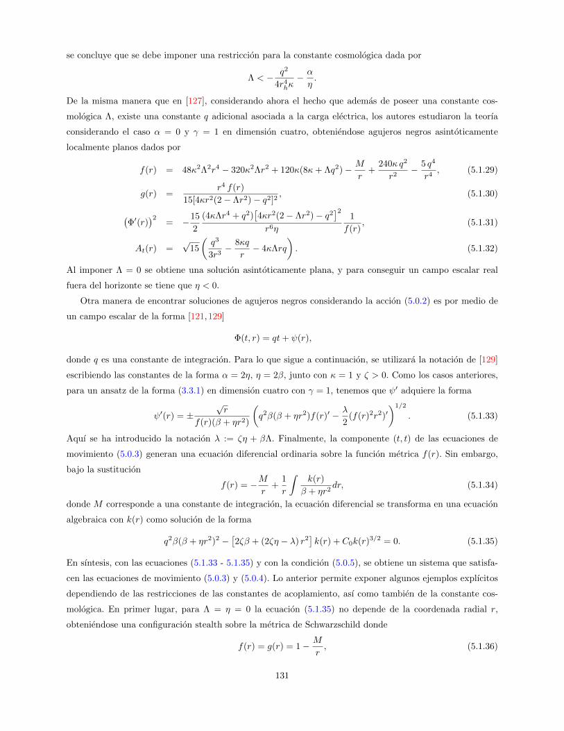
se concluye que se debe imponer una restriccion para la constante cosmologica dada por
Λ < − q2
4r4hκ− α
η.
De la misma manera que en [127], considerando ahora el hecho que ademas de poseer una constante cos-
mologica Λ, existe una constante q adicional asociada a la carga electrica, los autores estudiaron la teorıa
considerando el caso α = 0 y γ = 1 en dimension cuatro, obteniendose agujeros negros asintoticamente
localmente planos dados por
f(r) = 48κ2Λ2r4 − 320κ2Λr2 + 120κ(8κ+ Λq2)− M
r+
240κ q2
r2− 5 q4
r4, (5.1.29)
g(r) =r4 f(r)
15[4κr2(2− Λr2)− q2]2, (5.1.30)
(Φ′(r)
)2= −15
2
(4κΛr4 + q2)[4κr2(2− Λr2)− q2
]2
r6η
1
f(r), (5.1.31)
At(r) =√
15
(q3
3r3− 8κq
r− 4κΛrq
). (5.1.32)
Al imponer Λ = 0 se obtiene una solucion asintoticamente plana, y para conseguir un campo escalar real
fuera del horizonte se tiene que η < 0.
Otra manera de encontrar soluciones de agujeros negros considerando la accion (5.0.2) es por medio de
un campo escalar de la forma [121,129]
Φ(t, r) = qt+ ψ(r),
donde q es una constante de integracion. Para lo que sigue a continuacion, se utilizara la notacion de [129]
escribiendo las constantes de la forma α = 2η, η = 2β, junto con κ = 1 y ζ > 0. Como los casos anteriores,
para un ansatz de la forma (3.3.1) en dimension cuatro con γ = 1, tenemos que ψ′ adquiere la forma
ψ′(r) = ±√r
f(r)(β + ηr2)
(q2β(β + ηr2)f(r)′ − λ
2(f(r)2r2)′
)1/2
. (5.1.33)
Aquı se ha introducido la notacion λ := ζη + βΛ. Finalmente, la componente (t, t) de las ecuaciones de
movimiento (5.0.3) generan una ecuacion diferencial ordinaria sobre la funcion metrica f(r). Sin embargo,
bajo la sustitucion
f(r) = −Mr
+1
r
∫k(r)
β + ηr2dr, (5.1.34)
donde M corresponde a una constante de integracion, la ecuacion diferencial se transforma en una ecuacion
algebraica con k(r) como solucion de la forma
q2β(β + ηr2)2 −[2ζβ + (2ζη − λ) r2
]k(r) + C0k(r)3/2 = 0. (5.1.35)
En sıntesis, con las ecuaciones (5.1.33 - 5.1.35) y con la condicion (5.0.5), se obtiene un sistema que satisfa-
cen las ecuaciones de movimiento (5.0.3) y (5.0.4). Lo anterior permite exponer algunos ejemplos explıcitos
dependiendo de las restricciones de las constantes de acoplamiento, ası como tambien de la constante cos-
mologica. En primer lugar, para Λ = η = 0 la ecuacion (5.1.35) no depende de la coordenada radial r,
obteniendose una configuracion stealth sobre la metrica de Schwarzschild donde
f(r) = g(r) = 1− M
r, (5.1.36)
131

con M correspondiente a una constante de integracion. Ademas, el campo escalar es no trivial siendo de la
forma
Φ±(r) = qt± qM[
2
√r
M+ log
√r −√M√
r +√M
]+ Φ0, (5.1.37)
donde Φ0 es otra constante de integracion. Al escoger los parametros η 6= 0 y Λ 6= 0 junto con λ = ζη+βΛ = 0,
se encuentra una solucion donde las funciones metricas f(r) y g(r) adquieren la forma
f(r) = 1− M
r, g(r) =
(1− M
r
)(1 +
ηr2
β
), (5.1.38)
mientras que la parte radial del campo escalar Φ(t, r) esta dado por
ψ′(r) = ± q
f(r)
√M
r(1 + ηβ r
2), (5.1.39)
junto con la restriccion q2 = 2ζ/β. Un hecho interesante es considerar el caso f(r) = g(r), lo cual implica
que k(r) = (β+ηr2)2
β . Si lo anterior se complementa con las restricciones q2 = λ/(βη) y C0 = (2ζη−λ)√β/η,
se obtiene una solucion donde las funciones metricas toman la forma
f(r) = g(r) = 1− M
r+
η
3βr2, (5.1.40)
correspondientes a la metrica Schwarzschild-(A)dS expuesta en (3.3.2) para una constante cosmologica efec-
tiva Λeff = −ζη/β, ademas de
ψ′(r) = ± q
f(r)
√1− f(r). (5.1.41)
Como ultimo ejemplo, los autores en [129] estudian soluciones considerando un campo escalar estatico, esto
es q = 0, junto con C0 =√β(4ζ2η2 − λ2)/η, obteniendose una expresion para la funcion metrica f(r) dada
por
h(r) = 1− M
r+
η
3β
2ζη − λ2ζη + λ
r2 +λ2
4ζ2η2 − λ2
arctan(r√η/β)
r√η/β
, (5.1.42)
mientras que g(r) se obtiene por medio de las ecuaciones (5.0.5) y (5.1.42). La seccion radial del campo
escalar es de la forma(ψ′(r)
)2= − ζη3r2
(2ζβ + (2ζη − λ)r2
)2
β(4ζ2η2 − λ2)(β + ηr2)3f(r), (5.1.43)
la cual diverge en el horizonte de eventos.
5.2. Agujeros negros de Lifshitz con un campo escalar dependiente
del tiempo en una teorıa de Horndeski
A continuacion se analizaran soluciones de agujeros negros asintoticamente Lifshitz para una dimension
D arbitraria, presentes en el artıculo [5], considerando un ansatz metrico de la forma (4.0.3) y utilizando
como ecuacion fundamental la condicion (5.0.5) de manera de evadir el teorema de no-pelo expuesto en [124].
Bajo estas hipotesis, se prueba que no es posible hallar soluciones a las ecuaciones de movimiento (5.0.3)
y (5.0.4) para un campo escalar dependiente de la coordenada radial r. Sin embargo, logramos solucionar
este inconveniente agregando una dependencia temporal al campo escalar, obteniendose una solucion para
un valor particular del exponente dinamico z.
132

Lifshitz black holes with a time-dependent scalar field in a Horndeski theory
Moisés Bravo Gaete* and Mokhtar Hassaine†
Instituto de Matemática y Física, Universidad de Talca, Casilla 747, Talca, Chile(Received 21 April 2014; published 16 May 2014)
In arbitrary dimensions, we consider a particular Horndeski action given by the Einstein-HilbertLagrangian with a cosmological constant term, while the source part is described by a real scalar field withits usual kinetic term together with a nonminimal kinetic coupling. In order to evade the no-hair theorem,we look for solutions where the radial component of the conserved current vanishes identically. Under thishypothesis, we prove that this model cannot accommodate Lifshitz solutions with a radial scalar field. Thisproblem is finally circumvented by turning on the time dependence of the scalar field, and we obtain aLifshitz black hole solution with a fixed value of the dynamical exponent z ¼ 1
3. The same metric is also
shown to satisfy the field equations arising only from the variation of the matter source.
DOI: 10.1103/PhysRevD.89.104028 PACS numbers: 04.20.Jb, 04.50.Gh
I. INTRODUCTION
During the last decade, there has been intense activityto promote the ideas underlying the gauge-gravity dualityto nonrelativistic physics. The hope is to gain a betterunderstanding of some strongly coupled condensed matterphysics phenomena observed in laboratories, for a reviewsee, e.g., [1]. In this context, the so-called Schrödinger orLifshitz spacetimes are the natural candidates to be thegravity duals for nonrelativistic scale invariant theories,[2–4]. In the present work, we are concerned with theLifshitz spacetimes given by
ds2L ¼ −r2zdt2 þ dr2
r2þ r2d~x2D−2; (1)
where the dynamical exponent z reflects the anisotropy ofthe scaling symmetry
t → λzt; r →rλ; ~x → λ~x:
Here, ~x denotes a ðD − 2Þ-dimensional vector. As it is nowwell known, for z ≠ 1, in order for the Einstein gravity toaccommodate the Lifshitz spacetime, some extra mattersource is required, like p-form gauge fields or some Procamodel, see, e.g., [5]. There also exists the option ofconsidering higher-order gravity theories for which thereexist examples of Lifshitz black holes without source,see, e.g., [6,7]. By Lifshitz black holes, we mean a blackhole geometry whose asymptotic behavior reproduces theLifshitz spacetime (1). In this work, we deal with a sourceof the Einstein equations given by a real scalar field withits usual kinetic term together with a nonminimal kineticcoupling. More precisely, we consider the followingD-dimensional action
S¼Z ffiffiffiffiffiffi
−gp
dDxR−2Λ−
1
2ðαgμν−ηGμνÞ∇μϕ∇νϕ
; (2)
where R and Gμν stand, respectively, for the Ricci scalarand the Einstein tensor. This model is part of the so-calledHorndeski action which is the most general tensor-scalaraction yielding at most to second-order field equations infour dimensions [8]. The action also enjoys the shiftingsymmetry ϕ → ϕþ const. The field equations obtained byvarying the action with respect to the two dynamical fieldsgμν and ϕ read
Gμν þ Λgμν ¼1
2½αTð1Þ
μν þ ηTð2Þμν ; (3a)
∇μ½ðαgμν − ηGμνÞ∇νϕ ¼ 0; (3b)
where the stress tensors TðiÞμν are defined by
Tð1Þμν ¼
∇μϕ∇νϕ −
1
2gμν∇λϕ∇λϕ
:
Tð2Þμν ¼ 1
2∇μϕ∇νϕR − 2∇λϕ∇ðμϕRλ
νÞ −∇λϕ∇ρϕRμλνρ
− ð∇μ∇λϕÞð∇ν∇λϕÞ þ ð∇μ∇νϕÞϕþ 1
2Gμνð∇ϕÞ2
− gμν
−1
2ð∇λ∇ρϕÞð∇λ∇ρϕÞ
þ 1
2ðϕÞ2−∇λϕ∇ρϕRλρ
: (4)
The first exact black hole solution of these equationswithout the cosmological constant was found in [9].However, in this case, the scalar field becomes imaginaryoutside the horizon. Recently, this problem has beencircumvented by adding a cosmological constant termyielding to asymptotically locally (A)dS (and even flatfor α ¼ 0) black hole solutions with a real scalar fieldoutside the horizon [10]. The field equations (3) admit
*mbravog@inst‑mat.utalca.cl†hassaine@inst‑mat.utalca.cl
PHYSICAL REVIEW D 89, 104028 (2014)
1550-7998=2014=89(10)=104028(4) 104028-1 © 2014 American Physical Society
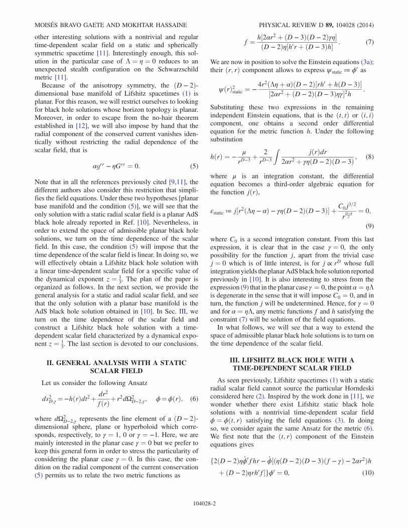
other interesting solutions with a nontrivial and regulartime-dependent scalar field on a static and sphericallysymmetric spacetime [11]. Interestingly enough, this sol-ution in the particular case of Λ ¼ η ¼ 0 reduces to anunexpected stealth configuration on the Schwarzschildmetric [11].Because of the anisotropy symmetry, the ðD − 2Þ-
dimensional base manifold of Lifshitz spacetimes (1) isplanar. For this reason, we will restrict ourselves to lookingfor black hole solutions whose horizon topology is planar.Moreover, in order to escape from the no-hair theoremestablished in [12], we will also impose by hand that theradial component of the conserved current vanishes iden-tically without restricting the radial dependence of thescalar field, that is
αgrr − ηGrr ¼ 0: (5)
Note that in all the references previously cited [9,11], thedifferent authors also consider this restriction that simpli-fies the field equations. Under these two hypotheses [planarbase manifold and the condition (5)], we will see that theonly solution with a static radial scalar field is a planar AdSblack hole already reported in Ref. [10]. Nevertheless, inorder to extend the space of admissible planar black holesolutions, we turn on the time dependence of the scalarfield. In this case, the condition (5) will impose that thetime dependence of the scalar field is linear. In doing so, wewill effectively obtain a Lifshitz black hole solution witha linear time-dependent scalar field for a specific value ofthe dynamical exponent z ¼ 1
3. The plan of the paper is
organized as follows. In the next section, we provide thegeneral analysis for a static and radial scalar field, and seethat the only solution with a planar base manifold is theAdS black hole solution obtained in [10]. In Sec. III, weturn on the time dependence of the scalar field andconstruct a Lifshitz black hole solution with a time-dependent scalar field characterized by a dynamical expo-nent z ¼ 1
3. The last section is devoted to our conclusions.
II. GENERAL ANALYSIS WITH A STATICSCALAR FIELD
Let us consider the following Ansatz
ds2D;γ ¼−hðrÞdt2þ dr2
fðrÞþ r2dΩ2D−2;γ; ϕ¼ϕðrÞ; (6)
where dΩ2D−2;γ represents the line element of a ðD − 2Þ-
dimensional sphere, plane or hyperboloid which corre-sponds, respectively, to γ ¼ 1, 0 or γ ¼ −1. Here, we aremainly interested in the planar case γ ¼ 0 but we prefer tokeep this general form in order to stress the particularity ofconsidering the planar case γ ¼ 0. In this case, the con-dition on the radial component of the current conservation(5) permits us to relate the two metric functions as
f ¼ h½2αr2 þ ðD − 3ÞðD − 2ÞγηðD − 2Þη½h0rþ ðD − 3Þh : (7)
We are now in position to solve the Einstein equations (3a);their ðr; rÞ component allows to express ψ static ≔ ϕ0 as
ψðrÞ2static ¼ −4r2ðΛηþ αÞðD − 2Þ½rh0 þ hðD − 3Þ
½2αr2 þ ðD − 2ÞðD − 3Þηγ2h :
Substituting these two expressions in the remainingindependent Einstein equations, that is the ðt; tÞ or ði; iÞcomponent, one obtains a second order differentialequation for the metric function h. Under the followingsubstitution
hðrÞ ¼ −μ
rD−3 þ2
rD−3
ZjðrÞdr
2αr2 þ γηðD − 2ÞðD − 3Þ ; (8)
where μ is an integration constant, the differentialequation becomes a third-order algebraic equation forthe function jðrÞ,
εstatic ≔ j½r2ðΛη − αÞ − γηðD − 2ÞðD − 3Þ þ C0j3=2
rD−42
¼ 0;
(9)
where C0 is a second integration constant. From this lastexpression, it is clear that in the case γ ¼ 0, the onlypossibility for the function j, apart from the trivial casej ¼ 0 which is of little interest, is for j ∝ rD whose fullintegrationyields theplanarAdSblackhole solution reportedpreviously in [10]. It is also interesting to stress from theexpression (9) that in the planar case γ ¼ 0, the point α ¼ ηΛis degenerate in the sense that it will impose C0 ¼ 0, and inturn, the function j will be undetermined. Hence, for γ ¼ 0and for α ¼ ηΛ, any metric functions f and h satisfying theconstraint (7) will be solution of the field equations.In what follows, we will see that a way to extend the
space of admissible planar black hole solutions is to turn onthe time dependence of the scalar field.
III. LIFSHITZ BLACK HOLE WITH ATIME-DEPENDENT SCALAR FIELD
As seen previously, Lifshitz spacetimes (1) with a staticradial scalar field cannot source the particular Horndeskiconsidered here (2). Inspired by the work done in [11], wewonder whether there exist Lifshitz static black holesolutions with a nontrivial time-dependent scalar fieldϕ ¼ ϕðt; rÞ satisfying the field equations (3). In doingso, we consider again the same Ansatz for the metric (6).We first note that the ðt; rÞ component of the Einsteinequations gives
f2ðD − 2Þη _ϕ0fhr − _ϕ½ðηðD − 2ÞðD − 3Þðf − γÞ − 2αr2Þhþ ðD − 2Þηrh0fgϕ0 ¼ 0; (10)
MOISÉS BRAVO GAETE AND MOKHTAR HASSAINE PHYSICAL REVIEW D 89, 104028 (2014)
104028-2
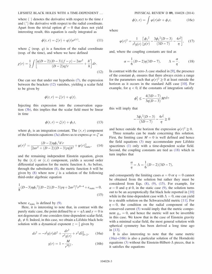
where ð .Þ denotes the derivative with respect to the time tand ð 0Þ the derivative with respect to the radial coordinate.Apart from the trivial option ϕ0 ¼ 0 that does not yieldinteresting result, this equation is easily integrated as
ϕðt; rÞ ¼ ζðrÞ þ qðtÞeχðrÞ; (11)
where ζ (resp. q) is a function of the radial coordinate(resp. of the time), and where we have defined
χðrÞ ¼ 1
2
Z ηðD − 2ÞðD − 3Þðf − γÞ − 2αr2
ðD − 2Þηfr þ h0
h
dr:
(12)
One can see that under our hypothesis (7), the expressionbetween the brackets (12) vanishes, yielding a scalar fieldto be given by
ϕðt; rÞ ¼ ζðrÞ þ qðtÞ:
Injecting this expression into the conservation equa-tion (3b), this implies that the scalar field must be linearin time
ϕðt; rÞ ¼ ζðrÞ þ ϕ1t; (13)
where ϕ1 is an integration constant. The ðr; rÞ componentof the Einstein equations (3a) allows us to express φ ≔ ζ0 as
φðrÞ2 ¼ ðD − 2Þηϕ12h0r
½2αr2 þ ðD − 2ÞðD − 3Þγηh2 þ ψðrÞ2static; (14)
and the remaining independent Einstein equation, givenby the ðt; tÞ or ði; iÞ component, yields a second orderdifferential equation for the metric function h. As before,through the substitution (8), the metric function h will begiven by (8) where now j is a solution of the followingthird-order algebraic equation
1
8ðD−3Þηϕ1
2½ðD−2ÞðD−3Þγηþ2αr22rD−4þ εstatic ¼ 0;
(15)
where εstatic is defined by (9).Here, it is interesting to note that, in contrast with the
purely static case, the point defined by α ¼ ηΛ and γ ¼ 0 isnot degenerate if one considers time-dependent scalar field,ϕ1 ≠ 0. Indeed, in this case, we obtain a Lifshitz black holesolution with a dynamical exponent z ¼ 1
3given by
ds2 ¼ −r23gðrÞdt2 þ dr2
r2gðrÞ þ r2d~x2D−2; (16a)
gðrÞ ¼ 1 −M
r3D−73
; (16b)
ϕðt; rÞ ¼Z
φðrÞdrþ ϕ1t; (16c)
where
φðrÞ2 ¼ 1
r83gðrÞ
ϕ1
2
gðrÞ −3ϕ1
2ðD − 3Þð3D − 7Þ −
4r23
η
; (17)
and, where the coupling constants are tied as
α ¼ 1
6ðD − 2Þηð3D − 7Þ; Λ ¼ α
η: (18)
In contrast with the zero-Λ case studied in [9], the presenceof the constant ϕ1 ensures that there always exists a rangefor the parameters such that φðrÞ2 ≥ 0 at least outside thehorizon as it occurs in the standard AdS case [10]. Forexample, for η < 0, if the constants of integration satisfy
ϕ21 ≤ −
4ð3D − 7Þ3ηðD − 3ÞM
23D−7
this will imply that
−3ϕ1
2ðD − 3Þð3D − 7Þ −
4r23
η≥ 0
and hence outside the horizon the expression φðrÞ2 ≥ 0.Three remarks can be made concerning this solution.
First, the limiting case M ¼ 0 is well defined and hencethe field equations (3) may accommodate pure Lifshitzspacetimes (1) only with a time-dependent scalar field.Second, the coupling constants are tied as (18) which inturn implies that
α
η¼ Λ ¼ 1
6ðD − 2Þð3D − 7Þ;
and consequently the limiting cases α ¼ 0 or η ¼ 0 cannotbe obtained from the solution but rather they must beconsidered from Eqs. (8), (9), (15). For example, forα ¼ 0 and η ≠ 0, in the static case (9), the solution turnsout to be an asymptotically flat black hole reported in [10]while in the time-dependent case with Λ ¼ 0, one can yieldto a stealth solution on the Schwarzschild metric [11]. Forη ¼ 0, the condition on the radial component of theconserved current (5) would imply that the metric compo-nent grr ¼ 0, and hence the metric will not be invertiblein this case. We know that in the case of Einstein gravitywith a minimal scalar field, the most general solution withspherical symmetry has been derived a long time agoin [13].It is also interesting to note that the same metric
(16a)–(16b) is also a particular solution of the Horndeskiequations (3) without the Einstein-Hilbert-Λ pieces, that isit satisfies the equations
LIFSHITZ BLACK HOLES WITH A TIME-DEPENDENT … PHYSICAL REVIEW D 89, 104028 (2014)
104028-3

αTð1Þμν þ ηTð2Þ
μν ¼ 0; (19)
provided that the scalar field is given by
ϕðt; rÞ ¼ ϕ1
ZφðrÞdrþ t
φðrÞ ¼ 1
fðrÞr43
ffiffiffiffiffiffiffiffiffiffiffiffiffiffiffiffiffiffiffiffiffiffiffiffiffiffiffiffiffiffiffiffiffiffiffiffiffiffiffiffiffiffiffiffiffiffiffiffiffiffiffiffi½ð3D − 7Þ − 3ðD − 3ÞfðrÞ
ð3D − 7Þ
s; (20)
and for the coupling constants given by (18).
IV. CONCLUSIONS
Here, we have considered a particular case of theHorndeski theory whose gravity theory is given by theEinstein piece and whose matter source is described by ascalar field with its usual kinetic term as well as anadditional nonminimal kinetic coupling. For this modeland for a static scalar field, we have shown that besides aplanar AdS black hole, this system cannot accommodateother solutions with a planar base manifold. In order tocircumvent this problem, we have seen that turning on thetime dependence of the scalar field is primordial to obtainLifshitz solutions. We have effectively derived a Lifshitzblack hole solution for a particular value of the dynamicalexponent z ¼ 1
3. There is a priori no physical reasons to
explain the occurrence of this particular value of thedynamical exponent. It will be interesting to see whetherother sectors of the Horndeski action may accommodatemore general Lifshitz solutions with other values of thedynamical exponents.We also believe that, because of the structure of the
solutions obtained in this paper as well as those derived in[9–11], the model considered here or maybe in moregeneral sectors of the Horndeski theory can be a good
laboratory in order to gain more insight concerning theblack hole solutions with scalar field. The task of findinginteresting solutions can also be explored for the recenttheory formulated in [14] and involving more than onescalar field but still yielding to second-order fieldequations.We would like to mention that the problem of stability of
the solution presented here is in some sense similar to whatoccurs in the case of the Bocharova-Bronnikov-Melnikov-Bekenstein solution in four dimensions [15,16]. Indeed, inthis case, the solution suffers from the fact that the scalarfield diverges at the horizon making its physical interpre-tation and the problem of its stability a subject of debate[17,18]. In the present case, in the action, the scalar fieldappears only through its derivatives and, its radial deriva-tive is unfortunately diverging at the horizon. Note thatthis also occurs for the AdS solutions [10]. Finally, thethermodynamics issue of our solution is also an openproblem because of its time-dependent character and alsobecause of its unusual asymptotic behavior (Lifshitz withdynamical exponent z ¼ 1=3). Future work to be done willconsist in providing a consistent Hamiltonian formalismthat accommodates the time-dependent character of thesolution in order to compute the mass, the entropy, and alsoto give a physical interpretation to the additional constantϕ1 that appears in the solution.
ACKNOWLEDGMENTS
We thank Julio Oliva for useful discussions. M. B. issupported by BECA DOCTORAL CONICYT 21120271.M. H. was partially supported by Grant No. 1130423 fromFONDECYT, by Grant No. ACT 56 from CONICYTand from CONICYT, Departamento de RelacionesInternacionales “Programa Regional MATHAMSUD 13MATH-05”.
[1] S. A.Hartnoll, ClassicalQuantumGravity26, 224002 (2009).[2] D. T. Son, Phys. Rev. D 78, 046003 (2008).[3] K. Balasubramanian and J. McGreevy, Phys. Rev. Lett. 101,
061601 (2008).[4] S. Kachru, X. Liu, and M. Mulligan, Phys. Rev. D 78,
106005 (2008).[5] D.-W. Pang, J. High Energy Phys. 01 (2010) 116.[6] E. Ayon-Beato, A. Garbarz, G. Giribet, and M. Hassaine,
Phys. Rev. D 80, 104029 (2009).[7] E. Ayon-Beato, A. Garbarz, G. Giribet, and M. Hassaine,
J. High Energy Phys. 04 (2010) 030.[8] G.W. Horndeski, Int. J. Theor. Phys. 10, 363 (1974).[9] M. Rinaldi, Phys. Rev. D 86, 084048 (2012).
[10] A. Anabalon, A. Cisterna, and J. Oliva, Phys. Rev. D 89,084050 (2014).
[11] E. Babichev and C. Charmousis, arXiv:1312.3204.[12] L. Hui and A. Nicolis, Phys. Rev. Lett. 110, 241104
(2013).[13] B. C. Xanthopoulos and T. Zannias, Phys. Rev. D 40, 2564
(1989).[14] A. Padilla, D. Stefanyszyn, and M. Tsoukalas, Phys. Rev. D
89, 065009 (2014).[15] N. M. Bocharova, K. A. Bronnikov, and V. N. Melnikov,
Vestn. Mosk. Univ., Ser. 3: Fiz., Astron. 6, 706 (1970)[Moscow Univ. Phys. Bull. 25, 80 (1970)].
[16] J. D. Bekenstein, Ann. Phys. (N.Y.) 91, 75 (1975).[17] K. A. Bronnikov and Y. N. Kireev, Phys. Lett. 67A, 95
(1978).[18] P. L. McFadden and N. G. Turok, Phys. Rev. D 71, 086004
(2005).
MOISÉS BRAVO GAETE AND MOKHTAR HASSAINE PHYSICAL REVIEW D 89, 104028 (2014)
104028-4
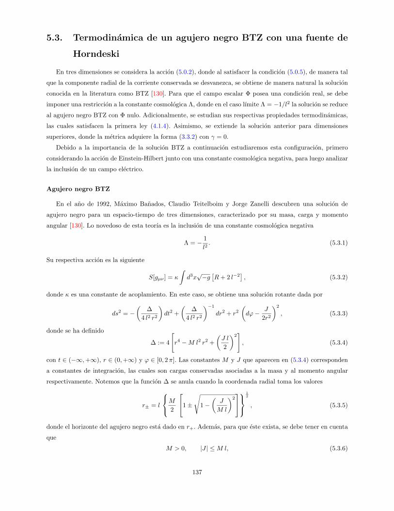
5.3. Termodinamica de un agujero negro BTZ con una fuente de
Horndeski
En tres dimensiones se considera la accion (5.0.2), donde al satisfacer la condicion (5.0.5), de manera tal
que la componente radial de la corriente conservada se desvanezca, se obtiene de manera natural la solucion
conocida en la literatura como BTZ [130]. Para que el campo escalar Φ posea una condicion real, se debe
imponer una restriccion a la constante cosmologica Λ, donde en el caso lımite Λ = −1/l2 la solucion se reduce
al agujero negro BTZ con Φ nulo. Adicionalmente, se estudian sus respectivas propiedades termodinamicas,
las cuales satisfacen la primera ley (4.1.4). Asimismo, se extiende la solucion anterior para dimensiones
superiores, donde la metrica adquiere la forma (3.3.2) con γ = 0.
Debido a la importancia de la solucion BTZ a continuacion estudiaremos esta configuracion, primero
considerando la accion de Einstein-Hilbert junto con una constante cosmologica negativa, para luego analizar
la inclusion de un campo electrico.
Agujero negro BTZ
En el ano de 1992, Maximo Banados, Claudio Teitelboim y Jorge Zanelli descubren una solucion de
agujero negro para un espacio-tiempo de tres dimensiones, caracterizado por su masa, carga y momento
angular [130]. Lo novedoso de esta teorıa es la inclusion de una constante cosmologica negativa
Λ = − 1
l2. (5.3.1)
Su respectiva accion es la siguiente
S[gµν ] = κ
∫d3x√−g
[R+ 2 l−2
], (5.3.2)
donde κ es una constante de acoplamiento. En este caso, se obtiene una solucion rotante dada por
ds2 = −(
∆
4 l2 r2
)dt2 +
(∆
4 l2 r2
)−1
dr2 + r2
(dϕ− J
2r2
)2
, (5.3.3)
donde se ha definido
∆ := 4
[r4 −M l2 r2 +
(J l
2
)2], (5.3.4)
con t ∈ (−∞,+∞), r ∈ (0,+∞) y ϕ ∈ [0, 2π]. Las constantes M y J que aparecen en (5.3.4) corresponden
a constantes de integracion, las cuales son cargas conservadas asociadas a la masa y al momento angular
respectivamente. Notemos que la funcion ∆ se anula cuando la coordenada radial toma los valores
r± = l
M
2
1±
√1−
(J
M l
)2
12
, (5.3.5)
donde el horizonte del agujero negro esta dado en r+. Ademas, para que este exista, se debe tener en cuenta
que
M > 0, |J | ≤M l, (5.3.6)
137
y para el caso extremo |J | = M l, ambas raıces coinciden.
De la solucion encontrada en (5.3.3) podemos obtener el estado vacıo, el cual corresponde al desvaneci-
miento de la solucion de agujero negro haciendo M → 0, lo cual implica de (5.3.6) que J → 0, obteniendose
ds2vacıo = −
(rl
)2
dt2 +(rl
)−2
dr2 + r2 dϕ2, (5.3.7)
donde la singularidad es desnuda. No obstante, existe un caso particular imponiendo las condiciones M = −1
y J = 0, permitiendo desaparecer este tipo de singularidad, sin la presencia de un horizonte de eventos
ds2 = −(
1 +r2
l2
)dt2 +
(1 +
r2
l2
)−1
dr2 + r2 dϕ2. (5.3.8)
Asimismo, los autores realizan un analisis de la solucion agregando el campo electrico a la accion (5.3.2),
donde la unica componente no nula del vector potencial viene dada por
At(r) = −Q log
(r
r0
), (5.3.9)
donde Q es una constante de integracion asociada a la carga electrica y definen r0 como un punto de referencia
arbitraria para la energıa. El elemento de lınea de esta nueva solucion es la siguiente
ds2 = −(
∆
4 l2 r2− 1
2Q2 log(r)
)dt2 +
(∆
4 l2 r2− 1
2Q2 log(r)
)−1
dr2 + r2
(dϕ− J
2r2
)2
, (5.3.10)
donde el horizonte de sucesos existe para cualquier valor de la constante Q, junto con la restriccion (5.3.6).
Por otra parte, al encontrar soluciones de agujero negros, para caracterizar cada una de las constantes de
integracion a los respectivos parametros termodinamicos resulta conveniente escribir la accion en su forma
Hamiltoniana [84]. Dado que para este caso en particular se estudiara una solucion estatica con un campo
escalar dependiente solamente de la coordenada radial r, se trabajara mediante el principio de accion reducida
IE = IG + IM +BE , (5.3.11)
donde IG e IM son las acciones asociadas a la gravitacion y a la fuente de materia respectivamente. Notemos
que el subındice E nos da a entender que la accion sera tomada considerando una metrica Euclideana, con
un tiempo Euclidiano dado por τ = it, el cual es periodico con perıodo β donde la temperatura de Hawking
esta dada por T = β−1. La clase de metrica Euclidiana en dimension D considerada aquı es la siguiente
ds20 = N(r)2 f(r) dτ2 +
dt2
f(r)+ r2dΣ2
D−2,0. (5.3.12)
Ademas, en la accion reducida (5.3.11) aparece una parametro BE , el cual es un termino de frontera que
es necesario sumar para que la accion Euclidiana tenga un extremo, esto es δIE = 0 [84]. Todo lo anterior
sera analizado a continuacion y corresponde al artıculo [6].
138

Thermodynamics of a BTZ black hole solution with a Horndeski source
Moises Bravo-Gaete* and Mokhtar Hassaine†
Instituto de Matemática y Física, Universidad de Talca, Casilla 747, Talca, Chile(Received 22 May 2014; published 1 July 2014)
In three dimensions, we consider a particular truncation of the Horndeski action that reduces to theEinstein-Hilbert Lagrangian with a cosmological constant Λ and a scalar field whose dynamics is governedby its usual kinetic term together with a nonminimal kinetic coupling. Requiring the radial component ofthe conserved current to vanish, the solution turns out to be the BTZ black hole geometry with a radialscalar field well defined at the horizon. This means in particular that the stress tensor associated to thematter source behaves on shell as an effective cosmological constant term. We construct a Euclidean actionwhose field equations are consistent with the original ones and such that the constraint on the radialcomponent of the conserved current also appears as a field equation. With the help of this Euclidean action,we derive the mass and the entropy of the solution, and find that they are proportional to thethermodynamical quantities of the BTZ solution by an overall factor that depends on the cosmologicalconstant. The reality condition and the positivity of the mass impose the cosmological constant to bebounded from above as Λ ≤ − 1
l2 where the limiting case Λ ¼ − 1l2 reduces to the BTZ solution with a
vanishing scalar field. Exploiting a scaling symmetry of the reduced action, we also obtain the usualthree-dimensional Smarr formula. In the last section, we extend all these results in higher dimensions wherethe metric turns out to be the Schwarzschild–anti–de Sitter spacetime with planar horizon.
DOI: 10.1103/PhysRevD.90.024008 PACS numbers: 04.50.Kd, 04.20.Jb, 04.50.-h
I. INTRODUCTION
Since the discovery of the BTZ black hole solution [1],three-dimensional Einstein gravity with a negative cosmo-logical constant has become an important field of inves-tigation. A considerable number of papers has been devotedto the physical and mathematical implications of the BTZsolution in particular in the context of AdS3=CFT2 corre-spondence. Indeed, it is now well accepted that three-dimensional gravity is an excellent laboratory in order toexplore and test some of the ideas behind the AdS=CFTcorrespondence [2].It is well known that the static BTZ geometry whose line
element is given by
ds2 ¼ −r2
l2−M
dt2 þ dr2
r2
l2 −Mþ r2dφ2 ð1Þ
is a solution of the Einstein equations with a fixed value ofthe negative cosmological constant −l−2,
Gμν − l−2gμν ¼ 0:
Here, we will exhibit a matter action that sources the BTZspacetime. In order to achieve this task, the correspondingstress tensor Tμν of the matter source must behave on shellas an effective cosmological constant term, i.e.
Ton shellμν ¼ ðl−2 þ ΛÞgμν:
Indeed, in this case, it is simple to realize that the Einsteinequations
Gμν þ Λgμν ¼ Tμν
will automatically be satisfied on the BTZ metric (1). Forthat purpose, we consider the following three-dimensionalaction
S ¼Z ffiffiffiffiffiffi
−gp
d3x
R − 2Λ −
1
2ðαgμν − ηGμνÞ∇μϕ∇νϕ
;
ð2Þ
where R and Gμν stand respectively for the Ricci scalar andthe Einstein tensor. This model is part of the so-calledHorndeski action which is the most general tensor-scalaraction yielding at most to second-order field equations infour dimensions [3]. In three dimensions, the correspond-ing field equations are also of second order, and aregiven by
Gμν þ Λgμν ¼1
2½αTð1Þ
μν þ ηTð2Þμν ; ð3aÞ
∇μ½ðαgμν − ηGμνÞ∇νϕ ¼ 0; ð3bÞ
where the stress tensors TðiÞμν are defined by
*mbravog@inst‑mat.utalca.cl†hassaine@inst‑mat.utalca.cl
PHYSICAL REVIEW D 90, 024008 (2014)
1550-7998=2014=90(2)=024008(7) 024008-1 © 2014 American Physical Society

Tð1Þμν ¼
∇μϕ∇νϕ −
1
2gμν∇λϕ∇λϕ
;
Tð2Þμν ¼ 1
2∇μϕ∇νϕR − 2∇λϕ∇ðμϕRλ
νÞ −∇λϕ∇ρϕRμλνρ
− ð∇μ∇λϕÞð∇ν∇λϕÞ þ ð∇μ∇νϕÞϕþ 1
2Gμνð∇ϕÞ2
− gμν
−1
2ð∇λ∇ρϕÞð∇λ∇ρϕÞ þ
1
2ðϕÞ2
−∇λϕ∇ρϕRλρ
: ð4Þ
The scalar field equation (3b) is a current conservationequation which is a consequence of the shift symmetry ofthe action, ϕ → ϕþ const.The first exact black hole solution of these equations
without cosmological constant was found in [4]. However,in this case, the scalar field becomes imaginary outside thehorizon. Indeed, in the notations of [4], α ¼ 1 and η ¼ zwith z proportional to the inverse of the graviton mass.In this case, the scalar field is given by
ðϕ0Þ2 ¼ −A2
zðm2p þ zÞ3FðrÞ ;
where A is a constant and mp is the Planck mass. However,considering the case with z > 0, the square of the derivativeof the scalar field becomes negative outside the horizon.Recently, this problem has been circumvented by adding acosmological constant term in [5] whose direct effect is thatone can have ðϕ0Þ2 > 0 outside the horizon with η ¼ z > 0by adjusting the sign of the cosmological constant yieldingto asymptotically locally (A)dS (and even flat for α ¼ 0)black hole solutions with a real scalar field outside thehorizon [5]. The electric charged version of the AdSsolutions has been studied in [6]. The field equations (3)admit other interesting solutions with a nontrivial andregular time-dependent scalar field on a static and spheri-cally symmetric spacetime [7]. Interestingly enough, thissolution in the particular case of Λ ¼ η ¼ 0 reduces to anunexpected stealth configuration on the Schwarzschildmetric [7]. There also exist Lifshitz black hole solutionswith a time-independent scalar field for a fixed value of thedynamical exponent z ¼ 1
3[8]. Solutions for a more general
truncation of the Horndeski action that is shift invariant aswell as enjoying the reflection symmetry ϕ → −ϕ havebeen obtained in [9]. In all these examples, in order to avoidthe no-hair theorem established in [10], the geometry hasbeen chosen such that
αgrr − ηGrr ¼ 0: ð5Þ
We note that this condition simplifies considerably thefield equations in particular in the time-independent casewhere the full conservation equation (3b) is automatically
satisfied without constraining the radial dependence ofthe scalar field.In the present work, we will show that the BTZ geometry
naturally emerges as a solution of this particular Horndeskiaction (2) in three dimensions subjected to the condition(5). We will also analyze the thermodynamical implicationsof such solution and extend all our results in arbitrarydimension. The plan of the paper is organized as follows.In the next section, we present in details the derivation ofthe solution using the constraint (5). In Sec. III, weconstruct a Euclidean action whose field equations turnout to be consistent with the original ones and such that theconstraint on the radial current (5) naturally appears as afield equation. This construction will be useful to obtain themass and the entropy of the solution. The usual Smarrformula is also derived by exploiting a scaling symmetry ofthe reduced action. The rotating version of the solution aswell as a particular example of a time-dependent solutionwill be reported in Sec. IV. In Sec. V, we extend all theresults to arbitrary dimension where the metric solution isnothing but the Schwarzschild-AdS spacetime with planarhorizon. The last section is devoted to our conclusions.
II. DERIVATION OF THE SOLUTION
Let us derive the most general solution of the fieldequations (3) subjected to the condition (5) with an ansatzof the form
ds2 ¼ −hðrÞdt2 þ dr2
fðrÞ þ r2dφ2;
ϕ ¼ ϕðrÞ: ð6Þ
For clarity, we define
ϵμν ≔ Gμν þ Λgμν −1
2½αTð1Þ
μν þ ηTð2Þμν :
The condition (5) on the geometry becomes
fðrÞ ¼ 2αrhðrÞηh0ðrÞ ; ð7Þ
and automatically implies that the current conservation (3b)is satisfied. Using this last relation, the radial component ofthe Einstein equations ϵrr ¼ 0 allows us to express thesquare of the derivative of the scalar field as
ðϕ0Þ2 ¼ −ðαþ ηΛÞh0
α2rh:
The remaining independent Einstein equation, ϵtt ¼ 0 orequivalently ϵφφ ¼ 0, yields
ϵtt ∝ ðα − ηΛÞ½rh00 − h0 ¼ 0:
MOISES BRAVO-GAETE AND MOKHTAR HASSAINE PHYSICAL REVIEW D 90, 024008 (2014)
024008-2
Hence, it is clear that the point defined by α ¼ ηΛcorresponds to a degenerate sector [8], while for α ≠ ηΛ,the solution is given by
hðrÞ ¼ Cr2 −M; fðrÞ ¼ α
ηCðCr2 −MÞ;
where C and M are two integration constants. In order todeal with the BTZ metric (1), we choose C ¼ l−2 and thecoupling constants must be fixed such that
α
η¼ l−2: ð8Þ
This means that the effective cosmological constant is fixedin terms of the coupling constants of the problem and doesnot correspond in general to the bulk cosmological con-stant. This is what differentiates our solution from the BTZone. Note also that the degenerate sector α ¼ ηΛ imposes achoice of the cosmological constant
Λdegenerate ¼ l−2: ð9Þ
In sum, for αη ¼ l−2 and Λ ≠ Λdeg, the solution is given by
the BTZ metric (1) together with a radial scalar field
ξðrÞ ≔ ðϕ0Þ2 ¼ −2ðΛl2 þ 1Þηðr2l2 −MÞ ; ð10aÞ
ϕðrÞ ¼ ffiffiffiffiffiffiffiffiffiffiffiffiffiffiffiffiffiffiffiffiffiffiffiffiffiffiffiffiffi−2l2ðΛl2 þ 1Þ
η
sln
0B@rlþ
ffiffiffiffiffiffiffiffiffiffiffiffiffiffir2
l2−M
s 1CA; ð10bÞ
provided that
2l2ðΛl2 þ 1Þη
≤ 0: ð11Þ
Various comments can be made concerning this solution.First, we note that for Λ ¼ −l−2, the scalar field vanishesidentically and the solution reduces to the BTZ solution.Second, the scalar field is well defined at the horizon rþ ¼l
ffiffiffiffiffiM
pand outside the horizon. Also, as expected the stress
tensor of the matter part behaves on shell as an effectivecosmological constant
1
2½αTð1Þ
μν þ ηTð2Þμν on shell ¼ ðΛþ l−2Þgμν: ð12Þ
We would like to stress that in the starting action, the scalarfield only appears through its derivative and hence oneshould worry about their regularity. However, it is easy to
see that the kinetic term grrðϕ0Þ2 as well as the nonminimalcoupling term Grrðϕ0Þ2 will be well defined at the horizonsince ðϕ0Þ2 ∝ grr [11]. As a last comment, we remark thatfor α > 0 which corresponds to the right sign of thestandard kinetic term, the previous reality conditions(8)–(11) will imply that η > 0 and the cosmologicalconstant Λ must be bounded from above as Λ ≤ −l−2.In the absence the cosmological constant, as it is the case in[4] and for η > 0, we do not have this freedom ðϕ0Þ2 < 0outside the horizon.In what follows, we will derive the mass and the entropy
of the solution (10).
III. THERMODYNAMICS OF THE BLACKHOLE SOLUTION
The partition function for a thermodynamical ensembleis identified with the Euclidean path integral in the saddlepoint approximation around the Euclidean continuation ofthe classical solution [12]. The Euclidean and Lorentzianaction are related by IE ¼ −iI where the periodicEuclidean time is τ ¼ it. The Euclidean continuation ofthe class of metrics considered here is given by [13]
ds2 ¼ N2ðrÞFðrÞdτ2 þ dr2
FðrÞ þ r2dφ2:
In order to avoid conical singularity at the horizon in theEuclidean metric, the Euclidean time is made periodic withperiod β and the Hawking temperature T is given byT ¼ β−1. Since we are only interested in a static solutionwith a radial scalar field, it is enough to consider a reducedaction principle. However, there is an important subtletythat has to do with the constraint (5) we used in order toderive our solution. Indeed, this constraint together with thefact of looking for a static scalar field make the equationassociated to the variation of the scalar field (3b) redundantin the sense that the equation is automatically satisfied.Hence, in our reduced action, the constraint (5) shouldappear as a field equation in order to deal with an equivalentproblem. This can be achieved considering the followingEuclidean action
IE ≔ IEðN;F; ξÞ ¼ 2πβ
Z∞
rþN
F0 þ 2Λrþ α
2rFξ
þ 3
4ηFF0ξþ η
2F2ξ0
drþ BE; ð13Þ
where the dynamical field is chosen to be ξðrÞ ≔ ðϕ0Þ2 andnot the scalar field itself ϕ. Note that rþ is the location ofthe horizon and BE is a boundary term that is fixed byrequiring that the Euclidean action has an extremum, that isδIE ¼ 0, [14]. In this case, the variation with respect to thedynamical fields N;F and ξ yield
THERMODYNAMICS OF A BTZ BLACK HOLE SOLUTION … PHYSICAL REVIEW D 90, 024008 (2014)
024008-3
EN ≔ F0 þ 2Λrþ α
2rFξþ 3
4ηFF0ξþ η
2F2ξ0 ¼ 0;
EF ≔ −N01þ 3
4ηFξ
þ N
α
2rξþ 1
4ηFξ0
¼ 0;
Eξ ≔ −η
2N0F2 þ N
α
2rF −
1
4ηF0F
¼ 0; ð14Þ
and the last equation Eξ ¼ 0 is nothing but the constraintused previously [(5)] to obtain our solution. At the specialpoint α ¼ η
l2, the equations (14) turn out to be equivalent tothe original ones supplemented by the constraint (5).Indeed, the most general solution of the system (14) canbe derived as follows. For XðrÞ ≔ 4þ 3ηFðrÞξðrÞ ≠ 0[15], we consider the combination
−2ηF2
XEF þ ηNF
XEN þ Eξ ¼ 0;
which permits us to obtain
ξðrÞ ¼ −2ðΛl2 þ 1Þ
ηFðrÞ :
Injecting this expression into EN ¼ 0, one obtains thatFðrÞ ¼ r2=l2 −M where M is an integration constant, andfinally the equation Eξ ¼ 0 implies thatN is constant whichcan be chosen to 1 without any loss of generality. Hence,at α ¼ η
l2, the most general solution of the system (14) isgiven by
NðrÞ ¼ 1; FðrÞ ¼ r2
l2−M; ξðrÞ ¼ −
2ðΛl2 þ 1ÞηFðrÞ ;
ð15Þ
and corresponds to the solution obtained previously [(10)].We now determine the boundary term of the Euclideanaction which is given by
δBE ¼ −2πβδF
1þ 3
4ηFξ
þ η
2F2δξ
∞
rþ: ð16Þ
In order to obtain δBE, we need the variations of the fieldsolutions (15) at infinity
δFj∞ ¼ −δM; ðF2δξÞj∞ ¼ 2ðΛl2 þ 1Þη
δFj∞;
while at the horizon, they are given by
δFjrþ ¼ −F0jrþδrþ ¼ −4π
βδrþ;
ðF2δξÞjrþ ¼ 2ðΛl2 þ 1Þη
δFjrþ ¼ −2ðΛl2 þ 1Þ
η
4π
βδrþ:
Hence, we have
IE ¼ BEð∞Þ − BEðrþÞ ¼ 2π½βM − 4πrþ1 − Λl2
2
;
and, we can identify the mass M and the entropy S of thesolution to be given by
M ¼ ∂IE∂β ; S ¼ β
∂IE∂β − IE;
yielding
M ¼ 2πM
1 − Λl2
2
; S ¼ 8π2
1 − Λl2
2
rþ: ð17Þ
Since the Hawking temperature is given by T ¼ 12π rþ, it is
easy to see that the first law dM ¼ TdS holds. In the BTZcase Λ ¼ −l−2, the scalar field vanishes and the mass andentropy reduce to the thermodynamical quantities of theBTZ solution [1].We can now go further by exploiting a scaling symmetry
of the reduced action in order to obtain the usual three-dimensional Smarr formula in the same lines as those donein Ref. [16]. In fact, it is easy to see that the reduced action(13) enjoys the following scaling symmetry
r ¼ σr; NðrÞ ¼ σ−2NðrÞ;FðrÞ ¼ σ2FðrÞ; ξðrÞ ¼ σ−2ξðrÞ; ð18Þ
from which one can derive a Noether quantity
CðrÞ ¼ N
1þ 3
4ηFξ
ð−2F þ rF0Þ þ η
2F2ðrξ0 þ 2ξÞ
;
which is conserved C0ðrÞ ¼ 0 by virtue of the fieldequations (14). Evaluating this quantity at infinity and atthe horizon, one gets
Cðr ¼ ∞Þ ¼ Mð1 − Λl2Þ;
Cðr ¼ rþÞ ¼4π
βrþ
1 − Λl2
2
:
Since the Noether charge is conserved, these expressionsmust be equal
Mð1 − Λl2Þ ¼ 4π
βrþ
1 − Λl2
2
;
which in turn implies the following Smarr formula
M ¼ T2S: ð19Þ
MOISES BRAVO-GAETE AND MOKHTAR HASSAINE PHYSICAL REVIEW D 90, 024008 (2014)
024008-4
This latter corresponds to the standard three-dimensionalSmarr formula [17].
IV. ROTATING, TIME-DEPENDENT ANDSTEALTH SOLUTIONS
Operating a Lorentz boost in the plane ðt;φÞ, we obtainthe rotating version of the solution found previously. At thepoint α ¼ ηl−2, the metric function turns out to be therotating BTZ
ds2 ¼ −FðrÞdt2 þ dr2
FðrÞ þ r2dφ −
J2r2
dt
2
; ð20Þ
where the structural function F is given by
FðrÞ ¼ r2
l2−M þ J2
4r2; ð21Þ
and, where J corresponds to the angular momentum.The scalar field solution reads
ξðrÞ ≔ ðϕ0ðrÞÞ2 ¼ −2ðl2Λþ 1Þ
ηFðrÞ : ð22Þ
We also report two solutions with a linear time scalarfield on the rotating BTZ metric (20). The first one isobtained for α ¼ ηl−2 and given by
ϕðt; rÞ ¼ qtZ ffiffiffiffiffiffiffiffiffiffiffiffiffiffiffiffiffiffiffiffiffiffiffiffiffiffiffiffiffiffiffiffiffiffiffiffiffiffiffiffiffiffiffi
q2η − 2FðrÞðΛl2 þ 1ÞηFðrÞ2
sdr; ð23Þ
where q is a constant. The second solution corresponds to astealth configuration, that is a solution where both sides ofthe Einstein equations (3a) vanish identically
Gμν þ Λgμν ¼ 0 ¼ 1
2½αTð1Þ
μν þ ηTð2Þμν : ð24Þ
In fact, for Λ ¼ −1=l2, a solution of the stealth equa-tions (24) is given by the rotating BTZ metric (20) togetherwith a time-dependent scalar field
ϕðt; rÞ ¼ qt
ZdrFðrÞ
; ð25Þ
where q is a constant. This stealth solution is different fromthe one derived in [18], where in this reference the authorsconsidered as a source a scalar field nonminimally coupledwhose action is given by
Z ffiffiffiffiffiffi−g
pd3x
R − 2Λ −
1
2∂μϕ∂μϕ −
ξ
2Rϕ2 −UðϕÞ
;
where U is a potential term involving power laws of ϕexpressed in terms of the nonminimal coupling parameter ξ.
Moreover, in [18], the time-dependent stealth only exists inthe case of the static BTZ metric, that is for J ¼ 0.
V. EXTENSION TO HIGHER DIMENSIONS
We now extend our analysis in arbitrary D dimensionswith the action
S ¼Z ffiffiffiffiffiffi
−gp
dDx
R − 2Λ −
1
2ðαgμν − ηGμνÞ∇μϕ∇νϕ
;
ð26Þ
for which the field equations are given by (3). Here, we willconsider an ansatz metric with a planar horizon and a staticradial scalar field
ds2 ¼ −N2Fdt2 þ dr2
Fþ r2d~x2D−2;
ϕ ¼ ϕðrÞ:
The solution of the field equations for this ansatz subjectedto the constraint (5) is now given by the Schwarzschild-AdS metric with a planar horizon
ds2 ¼ −FðrÞdt2 þ dr2
FðrÞ þ r2d~x2D−2; ð27aÞ
FðrÞ ¼ r2
l2−
MrD−3 ; ð27bÞ
ξðrÞ ≔ ðϕ0Þ2 ¼ −2ð2l2Λþ ðD − 1ÞðD − 2ÞÞ
ηðD − 1ÞðD − 2ÞFðrÞ ; ð27cÞ
provided that
α
η¼ ðD − 1ÞðD − 2Þ
2l2: ð28Þ
Note that as in the three-dimensional case, one can obtainan explicit expression of the scalar field
ϕðrÞ ¼ 2
ðD − 1Þ
ffiffiffiffiffiffiffiffiffiffiffiffiffiffiffiffiffiffiffiffiffiffiffiffiffiffiffiffiffiffiffiffiffiffiffiffiffiffiffiffiffiffiffiffiffiffiffiffiffiffiffiffiffiffiffiffiffiffi−2l2½2Λl2 þ ðD − 1ÞðD − 2Þ
ηðD − 1ÞðD − 2Þ
s
× ln
"rD−32
rlþ
ffiffiffiffiffiffiffiffiffiffiffiffiffiffiffiffiffiffiffir2
l2−
MrD−3
s #:
In the case D ¼ 3, the solution reduces to the onepreviously derived [(10)] on the BTZ spacetime, and inD ¼ 4, this solution was already reported in Ref. [5]. Asbefore, the stress tensor associated to the variation of thematter source behaves on shell as an effective cosmologicalconstant term, that is
THERMODYNAMICS OF A BTZ BLACK HOLE SOLUTION … PHYSICAL REVIEW D 90, 024008 (2014)
024008-5

1
2½αTð1Þ
μν þ ηTð2Þμν on shell ¼
Λþ ðD − 1ÞðD − 2Þ
2l2
gμν:
The reality condition (27c) together with the relation (28) and requiring the standard kinetic term to have the right signα > 0 impose the cosmological constant Λ to be bounded from above as
Λ ≤ −ðD − 1ÞðD − 2Þ
2l2: ð29Þ
The Euclidean action is now given by
IEðN;F; ξÞ ¼ βVolðΣD−2ÞZ
∞
rþN
ðD − 2ÞrD−3F0 þ 2ΛrD−2 þ α
2rD−2Fξþ 3ðD − 2Þ
4rD−3ηFF0ξ
þ ðD − 2Þη2
rD−3F2ξ0 þ ðD − 2ÞðD − 3ÞrD−4F þ η
4F2ξrD−4
drþ BE; ð30Þ
where VolðΣD−2Þ stands for the volume of the compactðD − 2Þ-dimensional planar manifold, and rþ ¼ðl2MÞ1=ðd−1Þ is the location of the horizon. The variationwith respect to the dynamical fields N;F and ξ yield
EN ≔ ðD − 2ÞrD−3F0 þ 2ΛrD−2 þ α
2rD−2Fξ
þ 3ðD − 2Þ4
rD−3ηFF0ξþ ðD − 2Þη2
rD−3F2ξ0
þ ðD − 2ÞðD − 3ÞrD−4F þ η
4F2ξrD−4
¼ 0;
EF ≔ −N0ðD − 2ÞrD−3 þ 3
4ðD − 2ÞrD−3ηFξ
þ N
α
2rD−2ξþ ðD − 2Þ
4rD−3ηFξ0
−ðD − 3ÞðD − 2Þ
4rD−4Fηξ
¼ 0;
Eξ ≔ −ðD − 2Þ
2ηrD−3N0F2
þ N
α
2rD−2F −
ðD − 2Þ4
rD−3ηFF0
−ðD − 3ÞðD − 2Þ
4rD−4F2η
¼ 0;
and the last equation Eξ ¼ 0 is again proportional to theconstraint (5) used previously to obtain the solution. Asbefore, at the special point (28), this system of equations isequivalent to our original equations supplemented by theconstraint (5) which also appears as a field equation. Themost general solution yields to (27) together with NðrÞ ¼ 1.We are now in position to compute the variation
δBE ¼ −βVolðΣD−2ÞðD − 2ÞrD−3
×
δF
1þ 3
4ηFξ
þ η
2F2δξ
∞
rþ; ð31Þ
which permits us to obtain that
IE ¼ ðD − 1ÞðD − 2Þ − 2l2Λ2ðD − 1Þ ½βM − 4πrD−2þ :
We derive the mass M ¼ ∂IE∂β and the entropy S ¼ β ∂IE∂β −IE that read
M ¼ðD − 1ÞðD − 2Þ − 2l2Λ
2ðD − 1ÞMVolðΣD−2Þ;
S ¼ðD − 1ÞðD − 2Þ − 2l2Λ
2ðD − 1Þ4πrD−2þ VolðΣD−2Þ; ð32Þ
and once again, one can easily check that the first lawholds. For the Schwarzschild-AdS case, that is forΛ ¼ − ðD−1ÞðD−2Þ
2l2 , these formulas reduce to those foundin [19]. Finally, the Noether conserved quantity
CðrÞ ¼ NrD−3ðD − 2Þ
1þ 3
4ηFξ
ð−2F þ rF0Þ
þ η
2F2ðrξ0 þ 2ξÞ
; ð33Þ
which is a consequence of the scaling symmetry of thereduced action (30)
r ¼ σr; NðrÞ ¼ σ1−DNðrÞ;FðrÞ ¼ σ2FðrÞ; ξðrÞ ¼ σ−2ξðrÞ ð34Þ
permits us to derive the following Smarr formula
M ¼ 1
D − 1TS: ð35Þ
One may mention that the previous scaling symmetry willnot be possible in the case of spherical or hyperboloidhorizon.
MOISES BRAVO-GAETE AND MOKHTAR HASSAINE PHYSICAL REVIEW D 90, 024008 (2014)
024008-6

VI. CONCLUSIONS
We have been concerned with a particular truncation ofthe Horndeski theory in three dimensions given by theEinstein-Hilbert piece plus a cosmological constant and ascalar field with its usual kinetic term and a nonminimalkinetic coupling. For this model, we have derived the mostgeneral solution subjected to the condition (5). In this case,the metric turns out to be the BTZ spacetime and the radialscalar field is shown to be well defined at the horizon. Wehave seen that such solution occurs because the stresstensor associated to the variation of the matter sourcebehaves on shell as a cosmological constant term. Theconstraint on the radial component of the conserved current(5) together with the fact of looking for a static scalar fieldonly impose a restriction on the geometry and not on thescalar field. In other words, this means that the fieldequation associated to the variation of the scalar field isautomatically satisfied without imposing any restriction onthe radial dependence of the scalar field. In order tocompute the mass and the entropy of the solution, wehave constructed a Euclidean action whose field equationsturn out to be equivalent to the original Einstein equationsand such that the constraint on the radial component of theconserved current appears also as a field equation. This lastfact has resulted to be primordial to obtain the mass andthe entropy, and we have verified that the first law wassatisfied. This reduced action has also been useful in orderto derive the usual Smarr formula by exploiting a scalingsymmetry. We have extended all these results in arbitrarydimension where the metric solution is nothing but theSchwarzschild-AdS spacetime with a planar horizon. Inthis case also, we have been able to construct an Euclideanaction whose field equations are equivalent to the originalones supplemented by the constraint condition on thegeometry (5). In all these examples, the horizon topology
is planar but this hypothesis is only essential in order toestablish a scaling symmetry of the reduced action. In fact,in the spherical or hyperboloid cases, one would be able toconstruct along the same lines the Euclidean action sharingthe same features except enjoying the scaling symmetry. Inhigher dimensions, the authors of Ref. [5] have considered the same model and found black hole solutions withspherical and hyperboloid horizon topology. In these cases,they have computed the thermodynamical quantities byregularizing the action with the use of a regular solitonsolution. It will be interesting to see whether the Euclideanapproach described here may yield the same results. It isalso appealing that up to now all the known solutions of theequations (3) are those where the constraint (5) is imposed.It will be interesting to see whether there exist othersolutions for which the radial component of the currentconservation is not vanishing. Finally, we have alsoobtained a particular time-dependent solution where thescalar field depends linearly on the time. For such solution,the issue concerning the thermodynamical analysis is notclear for us. Hence, a natural work will consist of providinga consistent Hamiltonian formalism in order to compute themass, the entropy and also to give a physical interpretationon the additional constant q that appears in the solution.This problem will also be relevant in the context of theLifshitz case where the known solutions [8,9] are neces-sarily time dependent.
ACKNOWLEDGMENTS
We thank Julio Oliva for useful discussions. M. B. issupported by BECA DOCTORAL CONICYT GrantNo. 21120271. M. H. is partially supported by GrantNo. 1130423 from FONDECYT and from CONICYT,Departamento de Relaciones Internacionales “ProgramaRegional MATHAMSUD 13 MATH-05.”
[1] M. Bañados, C. Teitelboim, and J. Zanelli, Phys. Rev. Lett.69, 1849 (1992).
[2] J. M. Maldacena, Adv. Theor. Math. Phys. 2, 231(1998).
[3] G.W. Horndeski, Int. J. Theor. Phys. 10, 363 (1974).[4] M. Rinaldi, Phys. Rev. D 86, 084048 (2012).[5] A. Anabalon, A. Cisterna, and J. Oliva, Phys. Rev. D 89,
084050 (2014).[6] A. Cisterna and C. Erices, Phys. Rev. D 89, 084038
(2014).[7] E. Babichev and C. Charmousis, arXiv:1312.3204.[8] M. Bravo-Gaete and M. Hassaine, arXiv:1312.7736.[9] T. Kobayashi and N. Tanahashi, arXiv:1403.4364.
[10] L. Hui and A. Nicolis, Phys. Rev. Lett. 110, 241104 (2013).[11] We thank the referee for pointing out this issue.
[12] G.W. Gibbons and S. W. Hawking, Phys. Rev. D 15, 2752(1977).
[13] For the ansatz considered in (6), this will correspond tohðrÞ ¼ NðrÞ2FðrÞ and fðrÞ ¼ FðrÞ.
[14] T. Regge and C. Teitelboim, Ann. Phys. (N.Y.) 88, 286(1974).
[15] For XðrÞ ¼ 0, one ends with a particular case of (10) with afixed value of the cosmological constant Λ ¼ − 1
3l2.[16] M. Banados and S. Theisen, Phys. Rev. D 72, 064019
(2005).[17] L. Smarr, Phys. Rev. Lett. 30, 71 (1973).[18] E. Ayon-Beato, C. Martinez, and J. Zanelli, Gen. Relativ.
Gravit. 38, 145 (2006).[19] D. Birmingham, Classical Quantum Gravity 16, 1197
(1999).
THERMODYNAMICS OF A BTZ BLACK HOLE SOLUTION … PHYSICAL REVIEW D 90, 024008 (2014)
024008-7
Capıtulo 6
Conclusiones y comentarios
En el capıtulo 3 se entregaron los conceptos fundamentales referentes a los artıculos [1, 2], considerando
una teorıa gravitatoria dada por una clase particular del Lagrangiano de Lovelock la cual puede ser vista como
una generalizacion de la gravedad de Einstein en dimension D arbitraria produciendo a lo mas ecuaciones
de segundo orden para la metrica. Esta clase particular de teorıa se encuentra caracterizada por un entero
k, fijando los coeficientes para obtener un unico vacıo AdS y asignando un valor particular a la constante
cosmologica. Inicialmente, comenzamos nuestro estudio considerando el caso particular k = 2 correspondiente
a la combinacion de la accion de Einstein-Hilbert con una constante cosmologica negativa junto con el termino
de Gauss-Bonnet, luego lo generalizamos para una accion arbitraria k ≥ 2.
Por otro lado, la parte asociada a la fuente de materia corresponde a un campo escalar no mınimamente
acoplado a la curvatura escalar, junto con un potencial dado por un termino de masa. Para este modelo
se derivaron dos clases de agujeros negros con una topologıa del horizonte de eventos planar, rotulados por
k y la dimension D, determinados por valores particulares del parametro de acoplamiento no minimal ξ.
La primera clase de solucion depende solamente de una constante de integracion, mientras que la segunda
depende de dos parametros y es interpretada como una configuracion stealth. Adicionalmente, se agrego a
la accion (D − 2)-campos, los cuales corresponden a (D − 1)-formas exactas acopladas al campo escalar,
logrando construir soluciones mas generales donde la constante de acoplamiento ξ es arbitraria. Cada una de
estas soluciones poseen su origen de una configuracion stealth sobre la metrica AdS dada en (3.3.3) a traves
de una transformacion de Kerr-Schild. Es importante tener en cuenta que estas soluciones son consideradas
para k ≥ 2, donde el caso particular k = 1 no puede ser obtenido por medio del mismo procedimiento, lo
que conlleva a la importancia de los terminos de curvatura superior en nuestras soluciones.
En [61,62], ademas de estudiar teorıas gravitatorias sin una fuente de materia, se estudiaron soluciones de
agujeros negros electricamente cargados considerando una fuente de Maxwell estandar (3.1.22). Es natural
cuestionarse si es posible encontrar versiones cargadas electricamente para las soluciones encontradas en [1,2].
Por otra parte, resulta interesante estudiar los efectos termodinamicos de esta clase de teorıa. Reciente-
mente, en [113] dan a conocer configuraciones mucho mas generales donde nuestros resultados corresponden
a un caso particular, concluyendo que tanto la masa como la entropıa se desvanecen.
En el capıtulo 4, en primer lugar se dieron los conceptos claves a los resultados presentes en [3], donde se
146

analizo una accion gravitatoria tridimensional dada por una teorıa caracterizada por una combinacion espe-
cial de las correcciones invariantes cuadraticas, conocida como nueva gravedad masiva, junto con una fuente
de materia asociada a un campo escalar no mınimamente acoplado y un potencial. Para este modelo, se
estudiaron las propiedades termodinamicas a tres diferentes clases de soluciones de agujeros negros asintoti-
camente Lifshitz. En particular, mediante el formalismo cuasilocal, el cual corresponde a una generalizacion
del metodo ADT, se obtuvieron las respectivas masas de estas soluciones, las cuales complementadas con la
entropıa de Wald (4.1.22) y la temperatura de Hawking (4.1.5) verificamos que se satisface la primera ley
de la termodinamica (4.1.4).
Por otro lado, para cada una de estas soluciones podemos encontrar sus homologos solitonicos. Mante-
niendo el mismo espıritu y mediante una transformacion adecuada de coordenadas, logramos calcular sus
masas corroborando la validez de la formula de Cardy generalizada, donde el estado fundamental es asumido
por la correspondiente solucion solitonica con masa Msol. Serıa interesante trabajar con la generalizacion
dimensional de estas soluciones, donde cada uno de los parametros termodinamicos se pueden obtener por
medio de un procedimiento similar [112].
En segundo lugar, dentro del mismo capıtulo se analizaron soluciones cargadas asintoticamente Lifshitz
presentes en [4] determinadas por la accion de Einstein-Hilbert con una constante cosmologica junto con las
correcciones de curvaturas cuadraticas mas generales, ademas de una fuente de materia correspondiente a un
campo de Maxwell lineal. Asimismo, a traves de ejemplos concretos confirmamos la validez del formalismo
cuasilocal propuesto en [92, 93]. De lo anterior es posible mostrar la existencia de cuatro clases de estas
soluciones, donde dos de ellas no requieren una restriccion para el exponente dinamico z. Tres de estos
agujeros negros cargados son interpretados como extremales en el sentido que la masa se desvanece mientras
que la carga electrica es no nula. Para la ultima familia, tanto la masa como la carga electrica dependen de
una unica constante de integracion. Para todos estos casos se muestra que la primera ley (4.1.4) se satisface.
En general, estas clases de soluciones son para una dimension D ≥ 5 debido a la presencia de un termino
adicional en las correcciones de curvaturas cuadraticas. No obstante, la solucion con masa no nula puede
reducirse al caso tridimensional donde la carga electrica se desvanece y obtenemos la masa del agujero negro
de Lifshitz para la teorıa gravitatoria nueva gravedad masiva [108] con z = 3.
En el capıtulo 5 se analizo un caso particular de la teorıa de Horndeski dada por la accion de Einstein-
Hilbert junto a un campo escalar con su respectivo termino cinetico y un termino cinetico no mınimamente
acoplado al tensor de Einstein. En particular, en [5] se estudio esta clase de teorıa considerando soluciones
de agujeros negros asintoticamente Lifshitz, llegado a la conclusion que la dependencia del campo escalar
respecto a la coordenada radial y temporal es esencial. Mas aun, cada una de estas soluciones se determinan
para un valor particular del exponente dinamico z = 1/3. Dado que solamente estamos trabajando un sector
de esta teorıa, serıa interesante considerar otros sectores de la accion de Horndeski los cuales permitan
extender las soluciones para otros valores del exponente dinamico.
Por otra parte, mirando desde el punto de vista termodinamico y dado que esta solucion posee una de-
pendencia temporal del campo escalar, queda como un problema abierto la construccion de un formalismo
que permita acomodar la caracterıstica temporal de la solucion y ası obtener parametros termodinamicos
tales como la masa y entropıa. Adicionalmente, en [6] se estudio la misma teorıa considerando en primer
147

lugar el caso particular tridimensional con un ansatz metrico dado en (3.3.1) con γ = 0, sujeta a la condi-
cion (5.0.5) donde se obtiene de manera natural la geometrıa del agujero negro BTZ junto con un campo
escalar dependiente de la coordenada radial, el cual es bien definido en el horizonte de eventos. Del mismo
modo, se extendieron estos resultados en dimension D-arbitraria cuya solucion corresponde a la metrica de
Schwarzschild-AdS con un horizonte planar dado en (3.3.2), estudiando sus respectivos parametros termo-
dinamicos mediante la construccion de una accion Euclidiana obteniendose la masa y la entropıa, verificando
que la primera ley de la termodinamica (4.1.4) se satisface. Asimismo, para el caso tridimensional se estu-
dio el caso rotante, logrando encontrar dos clases de soluciones, ambas dependientes del tiempo. Debido a
esta particularidad de dependencia temporal del campo escalar, aun no esta claro para nosotros el estudio
asociado a la termodinamica de estas soluciones, ası como tambien la existencia de agujeros negros con
momento angular para dimensiones superiores. Por ultimo, dado que tanto para [5] como [6] se considera la
condicion (5.0.5), serıa interesante encontrar soluciones, si es que existen, de tal manera que la componente
radial de la corriente conservada Jr de (5.0.4) no se desvanezca.
148

Capıtulo 7
Apendice
De manera tal que la seccion 4.5 sea lo mas clara posible, a continuacion daremos a conocer las distintas
expresiones para los coeficientes σij , ψij y ωij que aparecen en la ecuacion (4.5.12).
σ14 = −
2β1D2 + [(4 z − 10)β1 − 4β3 (1 + z)]D + 4β3 (2 z + 3) + 4β1(3− 2 z)− 1
/
2(z2 +D − 2
)= −σ24 = −2ψ23 = − 2
Dψ22 = 4ω22 = σ34 =
1
2(z +D + 1)σ33 = −4ω52,
σ13 =− 10β1D
3 + [(20β3 − 32β1) z + 50β1 + 16β3]D2 +[(20β3 − 20β1) z2 + (92β1 − 8β3) z
+5− 56β1 − 36β3]D + (−40β3 + 40β1) z2 + (−56β1 + 6− 88β3) z − 40β3 − 8β1 + 2
/4(z2 +D − 2
)= −σ23,
σ12 =− 8β1D
4 + [(16β3 − 36β1) z + 8β3 + 50β1]D3 +[(32β3 − 36β1) z2 + (132β1 + 12β3) z
−24β3 + 4− 86β1]D2 +[(16β3 − 16β1) z3 + (96β1 − 68β3) z2 + (10− 116β1 − 152β3) z
+28β1 − 4β3 − 1]D + (32β1 − 32β3) z3 + (2− 48β1) z2 + (56β3 − 8β1 − 2) z + 16β1
−16β3
/4(z2 +D − 2) = −σ22,
σ11 =− 2β1D
5 + [(4β3 − 12β1) z + 18β1]D4 +[(12β3 − 14β1) z2 + (60β1 + 16β3) z − 4β3
−50β1 + 1]D3 +[(20β3 − 8β1) z3 + (46β1 − 32β3) z2 + (4− 172β3 − 84β1) z + 16β3
−2 + 46β1]D2 +[(4β3 − 4β1) z4 + (20β1 − 104β3) z3 + (1− 24β1) z2 + (−10 + 376β3
+4β1) z + 1 + 4β1 − 28β3]D + (−8β3 + 8β1) z4 + (−6− 8β1 + 152β3) z3 + (−24β1 + 24β3) z2
+ (10 + 40β1 − 280β3) z − 16β1 + 16β3
/4(z2 +D − 2
)=
1
2(2−D)− σ21,
σ10 =[2β3(D − 3)(D − 4)− 1
]z (z +D − 2) ,
149

σ20 = −zβ3D3 −
[z β3 (z − 9) +
1
4
]D2 −
[z
(26β3 − 7 z β3 −
1
2
)− 3
4
]D −
(12β3 −
1
2
)z2
− (1− 24β3) z − 1
2= −σ50 −
1
2(D − 1)(D − 2),
ψ21 =
2β1D4 + [(−4β3 + 8β1) z − 18β1]D3 +
[(−6β1 − 4β3) z2 + (−8β3 − 28β1) z + 4β3 − 1
+50β1]D2 +[(−4β1 + 4β3) z3 + (26β1 + 44β3) z2 + (20β1 − 2 + 84β3) z − 12β3 + 2− 50β1
]D
+ (8β1 − 8β3) z3 + (−28β1 + 5− 92β3) z2 + (8β1 + 4− 104β3) z − 1 + 12β3 + 12β1
/
8 (z2 +D − 2),
σ32 =− 2β1D
4 + [(4β3 − 8β1)z + 6β1 + 4β3]D3 +[(8β3 − 6β1) z2 + (20β3 + 4β1) z − 12β3
+18β1 + 1]D2 +[(−8β1 + 8β3) z3 + (6β1 − 20β3) z2 + (64β1 − 84β3 + 2) z + 4β3
−66β1 + 2]D + (16β1 − 16β3) z3 + (12β3 − 1 + 12β1) z2 + (32β3 + 2− 80β1) z
−1 + 44β1 − 20β3
/2(z2 +D − 2
),
σ31 = −β1D
3 +[−2 z2β1 + (−8β3 + 9β1) z − 10β1 + 2β3
]D2 +
[2 (β1 − β3) z3 + (6β3 + 8β1) z2
+ (28β3 − 35β1) z − 1
2+ 27β1 − 8β3
]D + 4 (−β1 + β3) z3 +
(−1
2+ 34β1 − 22β3
)z
+ (1− 8β1 − 16β3) z2 +1
2− 22β1 + 10β3
(z +D − 1)
/(z2 +D − 2
),
σ30 = −(D − 2)(z − 1),
σ44 =− 2β1D
2 + [6β1 − 4 (β1 − β3) z + 8β3]D + 4 (−β1 + β3) z2 + 8 (β1 − β3) z − 20β3 − 4β1 + 1
/4(z2 +D − 2
)= −ψ53 + 2 (β3 − β1) ,
σ43 =− 2β1D
3 + [(4β3 − 6β1) z + 8β3 + 4β1]D2 +[(6β1 + 8β3) z − 8 (β1 − β3) z2 + 6β1 + 1
−16β3]D + (−8β1 + 8β3) z3 − 8 (β3 − β1) z2 + 1 + (12β1 + 1− 36β3) z − 12β3 − 12β1
/
2(z2 +D − 2
),
σ42 =− 2β1D
4 + [(4β3 − 8β1) z + 8β3 + 2β1]D3 +[(12β3 − 6β1) z2 + (40β3 − 24β1) z − 28β3
+1 + 34β1]D2 +[(20β3 − 20β1) z3 − 42 z2β1 + (2 + 152β1 − 116β3) z + 2− 86β1 + 24β3
]D
+ (20β3 − 20β1) z4 + (−8β3 + 8β1) z3 + (−32β3 + 104β1 − 3) z2 + (−144β1 + 6) z − 1
−28β3 + 52β1
/4(z2 +D − 2
),
150

σ41 =− 2β1D
4 +[8 z2β1 + (20β3 − 32β1) z − 8β3 + 26β1
]D3 +
[8 z3β1 + (20β3 − 94β1) z2
+ (−80β3 + 176β1) z + 36β3 + 1− 90β1]D2 +[(−60β1 + 4β3) z3 + (−40β3 + 262β1 − 4) z2
−56β3 + 118β1 + 2− 8 (β1 − β3) z4 + (2 + 84β3 − 312β1) z]D + 8 (−β1 + β3) z5
−4 (−β1 + β3) z4 + (13− 8β3 − 208β1) z2 + (88β1 + 8β3 − 8) z3 − 7 + (176β1 + 2− 32β3) z
+28β3 − 52β1
/4(z2 +D − 2
),
σ40 = −(z +D − 2) (z − 1),
σ52 = −1
2,
ψ52 =
6β1D3 + [(24β1 − 12β3) z − 46β1]D2 +
[(−104β1 + 20β3) z + 12 (β1 − β3) z2 + 100β1 − 3
]D
+12 (−β1 + β3) z3 + 28 (−β1 + β3) z2 − 64β1 + (32β3 + 112β1 − 6) z + 2 + 16β3
/
4(z2 +D − 2
),
ψ51 =
6β1D4 + [(32β1 − 12β3) z − 54β1]D3 +
[(−28β3 + 46β1) z2 + (32β3 − 204β1) z − 3
+174β1 − 12β3]D2 +[52β3 − 238β1 + 2 + (428β1 − 10 + 36β3) z + (76β3 − 202β1) z2
+12 (β1 − β3) z3]D + (16β3 − 16β1) z4 + 32 (−β1 + β3) z3 − 44β3 + (−12β3 + 228β1 − 13) z2
+116β1 + (16− 88β3 − 296β1) z + 5/
8(z2 +D − 2
),
ψ50 = −1
2
(3 z + 2D − 5
).
151

Bibliografıa
[1] M. Bravo Gaete and M. Hassaıne, Topological black holes for Einstein-Gauss-Bonnet gravity with a
nonminimal scalar field, Phys. Rev. D 88, 104011 (2013) [arXiv:1308.3076 [hep-th]].
[2] M. Bravo Gaete and M. Hassaıne, Planar AdS black holes in Lovelock gravity with a nonminimal scalar
field, JHEP 1311, 177 (2013) [arXiv:1309.3338 [hep-th]].
[3] E. Ayon-Beato, M. Bravo Gaete, F. Correa, M. Hassaıne, M. M. Juarez-Aubry and J. Oliva, First
law and anisotropic Cardy formula for three-dimensional Lifshitz black holes, Phys. Rev. D 91, 064006
(2015) [arXiv:1501.01244 [gr-qc]].
[4] M. Bravo Gaete and M. Hassaıne, Thermodynamics of charged Lifshitz black holes with quadratic co-
rrections, Phys. Rev. D 91, 064038 (2015) [arXiv:1501.03348 [hep-th]].
[5] M. Bravo Gaete and M. Hassaıne, Lifshitz black holes with a time-dependent scalar field in Horndeski
theory, Phys. Rev. D 89, 104028 (2014) [arXiv:1312.7736 [hep-th]].
[6] M. Bravo Gaete and M. Hassaıne, Thermodynamics of a BTZ black hole solution with an Horndeski
source, Phys. Rev. D 90, 024008 (2014) [arXiv:1405.4935 [hep-th]].
[7] A. Einstein, On the General Theory of Relativity, Sitzungsber. Preuss. Akad. Wiss. Berlin (Math. Phys.
) 1915 (1915) 778-786.
[8] A. Einstein, The Field Equations of Gravitation, Sitzungsber. Preuss. Akad. Wiss. Berlin (Math. Phys.
) 1915 (1915) 844-847.
[9] A. Einstein, The Foundation of the General Theory of Relativity, Annalen Phys. 49 (1916) 769-822.
[10] B. Janssen, Teorıa de la Relatividad General, Universidad de Granada, 2013.
[11] N. Straumann, The History of the cosmological constant problem, [gr-qc/0208027].
[12] S. Carroll, Spacetime and Geometry, an introduction to General Relativity, Addison Wesley, 2004.
[13] Hans Stephani, Dietrich Kramer, Malcolm MacCallum, Cornelius Hoenselaers, and Eduard Herlt, Exact
Solutions of Einstein’s Field Equations, Cambridge University Press, 2002.
[14] R. M. Wald, General Relativity, University of Chicago Press, 1984.
152
[15] K. Schwarzschild, On the gravitational field of a mass point according to Einstein’s theory, Sitzungsber.
Preuss. Akad. Wiss. Berlin (Math. Phys. ) 1916, 189 (1916) [physics/9905030].
[16] E. A. Larranaga, Agujeros Negros Clasicos, AshCat Publishers, 2011.
[17] H. Reissner, Uber die Eigengravitation des Elektrischen Feldes nach Einsteinschen Theorie, Ann. Phys.
59 (1916) 106-120.
[18] G. Nordstrom, On the Energy of the Gravitational Field in Einstein’s Theory, Proc. Kon. Ned. Akad.
Wet. 20 (1918) 1238-1245.
[19] R. P. Kerr, Gravitational field of a spinning mass as an example of algebraically special metrics, Phys.
Rev. Lett. 11, 237 (1963) 237-238.
[20] M. Visser, The Kerr spacetime: A Brief introduction, [arXiv:0706.0622 [gr-qc]].
[21] J. M. Maldacena, The Large N limit of superconformal field theories and supergravity, Int. J. Theor.
Phys. 38, 1113 (1999) [Adv. Theor. Math. Phys. 2, 231 (1998)] [hep-th/9711200].
[22] S. S. Gubser, I. R. Klebanov and A. M. Polyakov, Gauge theory correlators from noncritical string
theory, Phys. Lett. B 428, 105 (1998) [hep-th/9802109].
[23] E. Witten, Anti-de Sitter space and holography, Adv. Theor. Math. Phys. 2, 253 (1998) [hep-th/9802150].
[24] I. R. Klebanov and J. M. Maldacena, Solving quantum field theories via curved spacetimes, Phys. Today
62, 28 (2009).
[25] E. Papantonopoulos, From gravity to thermal gauge theories: The AdS/CFT correspondence, Lect. Notes
Phys. 828, 1 (2011).
[26] A. Einstein, Cosmological Considerations in the General Theory of Relativity, Sitzungsber. Preuss. Akad.
Wiss. Berlin (Math. Phys. ) 1917, 142 (1917).
[27] S. W. Hawking, Black holes in general relativity, Commun. Math. Phys. 25, 152 (1972).
[28] W. Israel, Event horizons in static vacuum space-times, Phys. Rev. 164, 1776 (1967).
[29] W. Israel, Event horizons in static electrovac space-times, Commun. Math. Phys. 8, 245 (1968).
[30] J. L. Friedman, K. Schleich and D. M. Witt, Topological censorship, Phys. Rev. Lett. 71, 1486 (1993)
[Erratum-ibid. 75, 1872 (1995)] [gr-qc/9305017].
[31] R. Emparan and H. S. Reall, A Rotating black ring solution in five-dimensions, Phys. Rev. Lett. 88,
101101 (2002) [hep-th/0110260].
[32] R. B. Mann, Pair production of topological anti-de Sitter black holes, Class. Quant. Grav. 14, L109
(1997) [gr-qc/9607071].
[33] L. Vanzo, Black holes with unusual topology, Phys. Rev. D 56, 6475 (1997) [gr-qc/9705004].
153

[34] D. R. Brill, J. Louko and P. Peldan, Thermodynamics of (3+1)-dimensional black holes with toroidal
or higher genus horizons, Phys. Rev. D 56, 3600 (1997) [gr-qc/9705012].
[35] D. Birmingham, Topological black holes in Anti-de Sitter space, Class. Quant. Grav. 16, 1197 (1999)
[hep-th/9808032].
[36] R. Ruffini and J. Wheeler, Introducing the Black Hole, Physics Today B24 (1971) 30.
[37] B. Carter, Axisymmetric Black Hole Has Only Two Degrees of Freedom, Phys. Rev. Lett. 26, 331 (1971).
[38] R. M. Wald, Final States of Gravitational Collapse, Phys. Rev. Lett. 26 (1971) 1653.
[39] D. C. Robinson, Uniqueness of the Kerr black hole, Phys. Rev. Lett. 34, 905 (1975).
[40] J. D. Bekenstein, Black holes: Classical properties, thermodynamics and heuristic quantization, [gr-
qc/9808028].
[41] N. M. Bocharova, K. A. Bronnikov and V. N. Melnikov, An exact solution of the system of Einstein
equations and mass-free scalar field, Vestn. Mosk. Univ. Fiz. Astron. 6 (1970) 706 [Moscow Univ. Phys.
Bull. 25 (1970) 80].
[42] J. D. Bekenstein, Exact Solutions Of Einstein Conformal Scalar Equations, Annals Phys. 82, 535 (1974).
[43] B.C. Xanthopoulos and T. Zannias,The uniqueness of the Bekenstein black hole, J. Math. Phys. 32,
1875 (1991).
[44] B.C. Xanthopoulos and T.E. Dialynas, Einstein gravity coupled to a massless conformal scalar field in
arbitrary space time dimensions, J. Math. Phys. 33, 1463 (1992).
[45] J. D. Bekenstein, Black Holes with Scalar Charge, Annals Phys. 91, 75 (1975).
[46] K. A. Bronnikov and Yu. N. Kireyev, Instability of Black Holes with Scalar Charge, Phys. Lett. A 67,
95 (1978).
[47] C. Martınez, R. Troncoso and J. Zanelli, De Sitter black hole with a conformally coupled scalar field in
four-dimensions, Phys. Rev. D 67, 024008 (2003) [hep-th/0205319].
[48] C. Martınez, J. P. Staforelli and R. Troncoso, Topological black holes dressed with a conformally coupled
scalar field and electric charge, Phys. Rev. D 74, 044028 (2006) [hep-th/0512022].
[49] E. Ayon-Beato, C. Martınez and J. Zanelli, Stealth scalar field overflying a (2+1) black hole, Gen. Rel.
Grav. 38, 145 (2006) [hep-th/0403228].
[50] A. Anabalon and A. Cisterna, Asymptotically (anti) de Sitter Black Holes and Wormholes with a Self
Interacting Scalar Field in Four Dimensions, Phys. Rev. D 85, 084035 (2012) [arXiv:1201.2008 [hep-th]].
[51] Y. Bardoux, M. M. Caldarelli and C. Charmousis, Shaping black holes with free fields, JHEP 1205, 054
(2012) [arXiv:1202.4458 [hep-th]].
154
[52] Y. Bardoux, M. M. Caldarelli and C. Charmousis, Conformally coupled scalar black holes admit a flat
horizon due to axionic charge, JHEP 1209, 008 (2012) [arXiv:1205.4025 [hep-th]].
[53] M. M. Caldarelli, C. Charmousis and M. Hassaıne, AdS black holes with arbitrary scalar coupling, JHEP
1310, 015 (2013) [arXiv:1307.5063 [hep-th]].
[54] C. Charmousis, Higher order gravity theories and their black hole solutions, Lect. Notes Phys. 769, 299
(2009) [arXiv:0805.0568 [gr-qc]].
[55] C. Lanczos, A Remarkable property of the Riemann-Christoffel tensor in four dimensions, Annals Math.
39, 842 (1938).
[56] D. Lovelock, The Einstein tensor and its generalizations, J. Math. Phys. 12, 498 (1971).
[57] C. Garraffo and G. Giribet, The Lovelock Black Holes, Mod. Phys. Lett. A 23, 1801 (2008) [ar-
Xiv:0805.3575 [gr-qc]].
[58] X. O. Camanho and J. D. Edelstein, A Lovelock black hole bestiary, Class. Quant. Grav. 30, 035009
(2013) [arXiv:1103.3669 [hep-th]].
[59] M. Banados, C. Teitelboim and J. Zanelli, Dimensionally continued black holes, Phys. Rev. D 49, 975
(1994) [gr-qc/9307033].
[60] R. G. Cai and K. S. Soh, Topological black holes in the dimensionally continued gravity, Phys. Rev. D
59, 044013 (1999) [gr-qc/9808067].
[61] J. Crisostomo, R. Troncoso and J. Zanelli, Black hole scan, Phys. Rev. D 62, 084013 (2000) [hep-
th/0003271].
[62] R. Aros, R. Troncoso and J. Zanelli, Black holes with topologically nontrivial AdS asymptotics, Phys.
Rev. D 63, 084015 (2001) [hep-th/0011097].
[63] D. G. Boulware and S. Deser, String Generated Gravity Models, Phys. Rev. Lett. 55, 2656 (1985).
[64] J. T. Wheeler, Symmetric Solutions to the Gauss-Bonnet Extended Einstein Equations, Nucl. Phys. B
268, 737 (1986).
[65] D. L. Wiltshire, Spherically Symmetric Solutions of Einstein-maxwell Theory With a Gauss-Bonnet
Term, Phys. Lett. B 169, 36 (1986).
[66] R. G. Cai, Gauss-Bonnet black holes in AdS spaces, Phys. Rev. D 65, 084014 (2002) [hep-th/0109133].
[67] G. T. Horowitz, Introduction to Holographic Superconductors, Lect. Notes Phys. 828, 313 (2011) [ar-
Xiv:1002.1722 [hep-th]].
[68] S. A. Hartnoll, C. P. Herzog and G. T. Horowitz, Holographic Superconductors, JHEP 0812, 015 (2008)
[arXiv:0810.1563 [hep-th]].
155

[69] C. P. Herzog, Lectures on Holographic Superfluidity and Superconductivity, J. Phys. A 42, 343001 (2009)
[arXiv:0904.1975 [hep-th]].
[70] V. Keranen and L. Thorlacius, Holographic geometries for condensed matter applications,
[arXiv:1307.2882[hep-th]].
[71] S. Kachru, X. Liu and M. Mulligan, Gravity Duals of Lifshitz-like Fixed Points, Phys. Rev. D 78, 106005
(2008) [arXiv:0808.1725 [hep-th]].
[72] D. W. Pang, On Charged Lifshitz Black Holes, JHEP 1001, 116 (2010) [arXiv:0911.2777 [hep-th]].
[73] A. Alvarez, E. Ayon-Beato, H. A. Gonzalez and M. Hassaıne, Nonlinearly charged Lifshitz black holes
for any exponent z > 1, JHEP 1406, 041 (2014) [arXiv:1403.5985 [gr-qc]].
[74] E. Ayon-Beato, A. Garbarz, G. Giribet and M. Hassaıne, Lifshitz Black Hole in Three Dimensions,
Phys. Rev. D 80, 104029 (2009) [arXiv:0909.1347 [hep-th]].
[75] E. Ayon-Beato, A. Garbarz, G. Giribet and M. Hassaıne, Analytic Lifshitz black holes in higher dimen-
sions, JHEP 1004, 030 (2010) [arXiv:1001.2361 [hep-th]].
[76] S. W. Hawking, Particle Creation by Black Holes, Commun. Math. Phys. 43, 199 (1975) [Erratum-ibid.
46, 206 (1976)].
[77] J. D. Bekenstein, Black holes and entropy, Phys. Rev. D 7, 2333 (1973).
[78] J. M. Bardeen, B. Carter and S. W. Hawking, The Four laws of black hole mechanics, Commun. Math.
Phys. 31, 161 (1973).
[79] E. Poisson : A Relativist’s Toolkit, The Mathematics of Black-Hole Mechanics, Cambridge University
Press, Cambridge (2004).
[80] R. M. Wald, Black hole entropy is the Noether charge, Phys. Rev. D 48, 3427 (1993) [gr-qc/9307038].
[81] V. Iyer and R. M. Wald, Some properties of Noether charge and a proposal for dynamical black hole
entropy, Phys. Rev. D 50, 846 (1994) [gr-qc/9403028].
[82] R. Wald, Quantum Field Theory in Curved Spacetime and Black Hole Thermodynamics, University of
Chicago Press, 1994.
[83] R. Arnowitt, S. Deser and C. Misner, The Dynamics of General Relativity, Phys. Rev. 116, 1322 (1959);
117, 1595 (1960); in Gravitation: An Introduction to Current Research, ed L. Witten (Wiley, New York,
1962).
[84] T. Regge, C. Teitelboim, Role of surface integrals in the Hamiltonian formulation of general relativity,
Annals Phys. 88, 286 (1974).
[85] E. Gourgoulhon, 3+1 formalism and bases of numerical relativity, [gr-qc/0703035].
156
[86] L. F. Abbott and S. Deser, Stability of Gravity with a Cosmological Constant, Nucl. Phys. B 195, 76
(1982).
[87] S. Deser and B. Tekin, Gravitational energy in quadratic curvature gravities, Phys. Rev. Lett. 89, 101101
(2002) [hep-th/0205318].
[88] S. Deser and B. Tekin, Energy in generic higher curvature gravity theories, Phys. Rev. D 67, 084009
(2003) [hep-th/0212292].
[89] S. Nam, J. D. Park and S. H. Yi, Mass and Angular momentum of Black Holes in New Massive Gravity,
Phys. Rev. D 82, 124049 (2010) [arXiv:1009.1962 [hep-th]].
[90] E. Witten, Anti-de Sitter space, thermal phase transition, and confinement in gauge theories, Adv.
Theor. Math. Phys. 2, 505 (1998) [hep-th/9803131].
[91] A. Bouchareb and G. Clement, Black hole mass and angular momentum in topologically massive gravity,
Class. Quant. Grav. 24, 5581 (2007) [arXiv:0706.0263 [gr-qc]].
[92] W. Kim, S. Kulkarni and S. H. Yi, Quasilocal Conserved Charges in a Covariant Theory of Gravity,
Phys. Rev. Lett. 111, no. 8, 081101 (2013) [Erratum-ibid. 112, 7, 079902 (2014)] [arXiv:1306.2138
[hep-th]].
[93] Y. Gim, W. Kim and S. H. Yi, The first law of thermodynamics in Lifshitz black holes revisited, JHEP
1407, 002 (2014) [arXiv:1403.4704 [hep-th]].
[94] D. O. Devecioglu and O. Sarioglu, Conserved Killing charges of quadratic curvature gravity theories in
arbitrary backgrounds, Phys. Rev. D 83, 021503 (2011) [arXiv:1010.1711 [hep-th]].
[95] D. O. Devecioglu and O. Sarioglu, On the thermodynamics of Lifshitz black holes, Phys. Rev. D 83,
124041 (2011) [arXiv:1103.1993 [hep-th]].
[96] S. Perlmutter et al. [Supernova Cosmology Project Collaboration], Measurements of Omega and Lambda
from 42 high redshift supernovae, Astrophys. J. 517, 565 (1999) [astro-ph/9812133].
[97] K. Hinterbichler, Theoretical Aspects of Massive Gravity, Rev. Mod. Phys. 84, 671 (2012) [ar-
Xiv:1105.3735 [hep-th]].
[98] I. Gullu, Massive Higher Derivative Gravity Theories, [arXiv:1201.6504 [gr-qc]].
[99] A. G. Riess et al. [Supernova Search Team Collaboration], Observational evidence from supernovae for
an accelerating universe and a cosmological constant, Astron. J. 116, 1009 (1998) [astro-ph/9805201].
[100] S. Weinberg, The Quantum theory of fields. Vol. 1: Foundations, Cambridge, UK: Univ. Pr. (1995) 609
p
[101] M. Fierz and W. Pauli, On relativistic wave equations for particles of arbitrary spin in an electromag-
netic field, Proc. Roy. Soc. Lond. A 173, 211 (1939).
157

[102] W. Pauli and M. Fierz, On Relativistic Field Equations of Particles With Arbitrary Spin in an Elec-
tromagnetic Field, Helv. Phys. Acta 12, 297 (1939).
[103] S. Deser, R. Jackiw and S. Templeton, Topologically Massive Gauge Theories, Annals Phys. 140, 372
(1982) [Erratum-ibid. 185, 406 (1988)] [Annals Phys. 185, 406 (1988)] [Annals Phys. 281, 409 (2000)].
[104] S. Deser, R. Jackiw and S. Templeton, Three-Dimensional Massive Gauge Theories, Phys. Rev. Lett.
48, 975 (1982).
[105] W. Li, W. Song and A. Strominger, Chiral Gravity in Three Dimensions, JHEP 0804, 082 (2008)
[arXiv:0801.4566 [hep-th]].
[106] S. Deser and B. Tekin, Energy in topologically massive gravity, Class. Quant. Grav. 20, L259 (2003)
[gr-qc/0307073].
[107] S. Olmez, O. Sarioglu and B. Tekin, Mass and angular momentum of asymptotically ads or flat solutions
in the topologically massive gravity, Class. Quant. Grav. 22, 4355 (2005) [gr-qc/0507003].
[108] E. A. Bergshoeff, O. Hohm and P. K. Townsend, Massive Gravity in Three Dimensions, Phys. Rev.
Lett. 102, 201301 (2009) [arXiv:0901.1766 [hep-th]].
[109] K. S. Stelle, Renormalization of Higher Derivative Quantum Gravity, Phys. Rev. D 16, 953 (1977).
[110] K. S. Stelle, Classical Gravity with Higher Derivatives, Gen. Rel. Grav. 9, 353 (1978).
[111] Y. Liu and Y. w. Sun, Note on New Massive Gravity in AdS(3), JHEP 0904, 106 (2009) [ar-
Xiv:0903.0536 [hep-th]].
[112] E. Ayon-Beato, M. Bravo Gaete, F. Correa, M. Hassaıne, M. M. Juarez-Aubry, J. Oliva, work in
progress.
[113] F. Correa and M. Hassaıne, Thermodynamics of Lovelock black holes with a nonminimal scalar field,
JHEP 1402, 014 (2014) [arXiv:1312.4516 [hep-th]].
[114] J. Oliva, D. Tempo and R. Troncoso, Three-dimensional black holes, gravitational solitons, kinks and
wormholes for BHT massive gravity, JHEP 0907, 011 (2009) [arXiv:0905.1545 [hep-th]].
[115] F. Correa, M. Hassaıne and J. Oliva, Black holes in New Massive Gravity dressed by a (non)minimally
coupled scalar field, Phys. Rev. D 89, 124005 (2014) [arXiv:1403.6479 [hep-th]].
[116] V. Belinski and E. Verdaguer, Gravitational Solitons, Cambridge University Press, 2005.
[117] F. Correa, C. Martınez and R. Troncoso, Scalar solitons and the microscopic entropy of hairy black
holes in three dimensions, JHEP 1101, 034 (2011) [arXiv:1010.1259 [hep-th]].
[118] H. A. Gonzalez, D. Tempo and R. Troncoso, Field theories with anisotropic scaling in 2D, solitons and
the microscopic entropy of asymptotically Lifshitz black holes, JHEP 1111, 066 (2011) [arXiv:1107.3647
[hep-th]].
158
[119] G. W. Horndeski, Second-order scalar-tensor field equations in a four-dimensional space, Int. J. Theor.
Phys. 10, 363 (1974).
[120] C. Deffayet, S. Deser and G. Esposito-Farese, Generalized Galileons: All scalar models whose curved
background extensions maintain second-order field equations and stress-tensors, Phys. Rev. D 80, 064015
(2009) [arXiv:0906.1967 [gr-qc]].
[121] C. Charmousis, From Lovelock to Horndeski’s generalised scalar-tensor theory, Lect. Notes Phys. 892,
25 (2015) [arXiv:1405.1612 [gr-qc]].
[122] T. Kobayashi, M. Yamaguchi and J. Yokoyama, Generalized G-inflation: Inflation with the most general
second-order field equations, Prog. Theor. Phys. 126, 511 (2011) [arXiv:1105.5723 [hep-th]].
[123] T. Kobayashi and N. Tanahashi, Exact black hole solutions in shift symmetric scalar-tensor theories,
PTEP 2014, n 7, 073E02 (2014) [arXiv:1403.4364 [gr-qc]].
[124] L. Hui and A. Nicolis, No-Hair Theorem for the Galileon, Phys. Rev. Lett. 110, n 24, 241104 (2013)
[arXiv:1202.1296 [hep-th]].
[125] M. Rinaldi, Black holes with non-minimal derivative coupling, Phys. Rev. D 86, 084048 (2012) [ar-
Xiv:1208.0103 [gr-qc]].
[126] S. W. Hawking and D. N. Page, Thermodynamics of Black Holes in anti-De Sitter Space, Commun.
Math. Phys. 87, 577 (1983).
[127] A. Anabalon, A. Cisterna and J. Oliva, Asymptotically locally AdS and flat black holes in Horndeski
theory, Phys. Rev. D 89, 084050 (2014) [arXiv:1312.3597 [gr-qc]].
[128] A. Cisterna and C. Erices, Asymptotically locally AdS and flat black holes in the presence of an electric
field in the Horndeski scenario, Phys. Rev. D 89, no. 8, 084038 (2014) [arXiv:1401.4479 [gr-qc]].
[129] E. Babichev and C. Charmousis, Dressing a black hole with a time-dependent Galileon, JHEP 1408,
106 (2014) [arXiv:1312.3204 [gr-qc]].
[130] M. Banados, C. Teitelboim and J. Zanelli, The Black hole in three-dimensional space-time, Phys. Rev.
Lett. 69, 1849 (1992) [hep-th/9204099].
159