THE JOINT DISTRIBUTION OF DOMESTIC INDEXES. AN … · Kopulen teoria interes handikoa da aktiboen arteko baterako banaketa funtzioa aztertzerako orduan, bereziki VaR (Value at Risk)

THE JOINT DISTRIBUTION OF DOMESTIC

INDEXES. AN APPROACH USING

CONDITIONAL COPULAS

Jone Ascorbebeitia Bilbatua

Trabajo de investigación 013/016

Master en Banca y Finanzas Cuantitativas

Tutores: Dra. Eva Ferreira

Dra. Susan Orbe-Mandaluniz

Universidad Complutense de Madrid

Universidad del País Vasco

Universidad de Valencia

Universidad de Castilla-La Mancha

www.finanzascuantitativas.com

The Joint Distribution of Domestic Indexes.An Approach Using Conditional Copulas

Jone Ascorbebeitia BilbatuaMaster’s Degree in Banking and Quantitative Finance

Supervisors:Eva Ferreira*

Susan Orbe-Mandaluniz ∗

Sarrera

Finantza-aktiboak askotan erlazionatuta egoten dira eta erlazio horreek garrantzi handikoak izan daitekez.Izan ere, finantza-aktiboek euren artean daukiezan erlazioen analisia oso interesgarria da Ekonomia eta Fi-nantza arloetan. Zorroek, aktiboek eta baita indizeek ere aldaketak jasotzen dabez egunero euren balioetaneta ondorioz aktiboen arteko erlazioak ere aldaketen eragina izan daikie. Aldaketak edozein unetan eta arrazoidesberdinengatik gertatu daitekez. Baliteke zorroen arteko mugimenduak denborarekin aldatzearen ondoriozemotea. Literaturan badagoz gertakizun hau balioztatzen daben lan desbardinak, esaterako Krishnan, Petkovaeta Ritchken (2009), Ferreira, Gil eta Orbe (2011) eta Ferreira eta Orbek (“Why are there time-varying co-movements in the European stock market?”(2015)) argitaratutako lanak. Guk mugimenduen aldakuntza zen-bait arrisku faktore globalen bitartez azaldu daitekeen aurkitu nahi dogu, hala nola, indize global baten bidezadierazitako merkatu faktore bat. Gainera, korrelazio lineala baino haratago doazen menpekotasun neurriakinteresatzen jakuz.

Lan honetan Europar herrialdeetako indizeen arteko erlazioetan zentratuko gara. Ezaguna danez, indizeenartean dagoen menpekotasuna nabaria dala eta menpekotasun horren zati bat Euro Stoxx indizearen bitartezazalduta egon beharko leuke.

Beraz, indize global batekin herrialdeetako indize desberdinen analisiak interes esanguratsua dauka Ekono-mia eta Finantza arloetako aspektu batzuetan. Ohituta gagoz korrelazio lineala neurtzen dauan Pearsonenkorrelazio koefizientea kalkulatzen, baina zer gertatzen da indizeen arteko menpekotasuna erlazio lineal batenbidez ez badator? Pearsonen korrelazio koefizientea kalkulatzeko ez ezik interpretatzeko ere erraza da, bainabaliteke nahikoa ez izatea. Menpekotasun neurri aproposa da banaketa normala jarraitzen daben aldagaietarakobaina ez normala izatetik urruti dagozan aldagaietarako. Izan ere, finantza aldagaien arteko erlazioak konplikat-uagoak izan daitekez eta hori dala eta orokorragoa dan beste zerbait beharrezkoa da. Sarritan, zorroen akti-boetako errentagarritasunen banaketa funtzio marjinalak desberdinak izaten dira, baita asimetrikoak edo muturhandietakoak ere eta egoera honeetan korrelaziokoefiziente lineala ez da neurri egokia. Orduan, menpekotasunegitura kopula deituriko funtzio batzuen bitartez modelizatu daiteke. Kopulak baterako banaketa funtzioak diraeta banaketa funtzio marginalak bateratzea ahalbidetzen dabe. Beraz, kopula eta banaketa funtzio marginalenbitartzez aldagaien baterako banaketa funtzioa definitu daiteke. Banaketa funtzio marjinalak baterako banaketa

∗UPV/EHU University of Basque Country

funtzioa baino modelizatzeko errazagoak izateak abantaila bat suposatzen dau. Kopulen teoria interes handikoada aktiboen arteko baterako banaketa funtzioa aztertzerako orduan, bereziki VaR (Value at Risk) (John C. Hull(2012), Jorion (2003) and Parra and Koodi (2006) among others) bezalako neurriak kalkulatzerako orduan.

Arrazoi honeek direla eta, kopulen bitartez herrialde desberdinetako indizeen arteko erlazioa aztertuko dogueta baita, kopula baldintzatuak erabiliz, indize globalari (Euro Stoxx) baldintzatutako erlazioak ere. Gainera,menpekotasuna eta baldintzatutako menpekotasuna neurtuko doguz korrelazio koefiziente linealaren ezberdinakdiren Kendall-en tau koefizientea bezalako beste neurri batzuekin.

Aipatu bezala, analisi enpirikoan Europar indizeetako erlazioan zentratuko gara. Zehatz-mehatz hurrengoherrialdeetako indizeen eguneroko datuak erabiliko doguz: Espainia (IBEX 35), Frantzia (CAC 40), Alemania(DAX), Erresuma batua (FTSE 100) eta suitza (SMI). Indize global moduan Euro Stoxx (EUROSTOXX 50)indizea erabiliko dogu.

Artikulua bost zatitan egituratuta dago. Lehenengo atalean baldintztutako kopulak estimatzeko prozeduradeskribatzen da. Bigarren atalean Euro Stoxx-arekiko menpekotasuna aztertzen da. Kopulen teorian azaltzendiran menpekotasun neurriak azaltzeaz gain, neurri desberdinen arteko desberdintasunak eztabaidatuko dira.Hirugarren atalean aukeratutako neurriarekin (Kendall-en tau koefizientea) menpekotasunaren testa burutukodogu. Behin jakinda indizeen artean menepekotasuna dagoela, laugarren atalean erregresio eredu ez-parametrikobat proposatzen dogu eta hurrengo galdera erantzuten saiatuko gara: Ba al dago inolako menpekotasun gehigar-ririk jatorrizko aldagaietatik Euro Stoxx-arekiko batazbesteko menpekotasuna kenduz gero? Azkenik, lortutakoemaitzak errazagoa dan erregresio linealaren bidez lortutako emaitzekin konparatuko doguz. Bosgarren atalaondorioen atalari dagokio.

2

Introduction

The analysis of relationships between financial assets is a topic of great interest in Economics and Finance.Every day, portfolios, assets or indexes undergo changes and the relationship between them might also beaffected. It is well known that the comovements between portfolios are time-varying. This fact is supported byworks as, among others, Krishnan, Petkova and Ritchken (2009), Ferreira, Gil and Orbe (2011) and Ferreiraand Orbe (2015). Our interest is to detect whether these comovements variation can be explained by someglobal risk factors as a market factor represented by a global index. Moreover, we are interested in measures ofdependece beyond linear correlation.

We are going to focus on the relation between domestic European indexes. It’s known that there is a greatdependence between domestic indexes and that part of this dependence should be explained by Euro Stoxxindex.

So, the analysis of domestic indexes with global indexes has a significant interest for some aspects in Eco-nomics and Finance. We are used to calculate the Pearson’s correlation coefficient, which measures linearcorrelation, but what if the dependence between indexes is not given by a linear relationship? Pearson’s corre-lation coefficient is very intuitive and easy to calculate but this might not be enough. It is a perfect measure ofdependence for normal variables but not for variables are far from being normal distributed. In fact, relation-ships between financial variables can be more complicated and that’s why something more general is needed.In addition, many times marginal distributions of assets returns of a portfolio are different, asymmetric or havebig tails and in those situations the linear correlation coefficient is not the adequate measure. Then, one way tomodel the dependence structure is through functions called copulas, which allow constructing a joint distributionfunction to represent de returns dependence better than an elliptic distribution. Copulas allow for obtaining,together with marginal distribution function, the joint distribution function. An advantage comes from the factthat marginal distribution functions are always easier modelling than the joint distribution. Copula theory hasa high interest while studying the joint probability distribution function between assets, particularly to obtainmeasures such as VaR (Value at Risk) (John C. Hull (2012), Jorion (2003) and Parra and Koodi (2006) amongothers).

For these reasons, we will study the relation between domestic indexes using copulas, and the relation condi-tioned to the global index (Euro Stoxx), using conditional copulas. Moreover, we will measure the dependenceand the conditional dependence using other measures than the linear correlation, as the Kendall’s tau.

As we have mentioned before, for the empirical analysis we will focus on the relationships between Europeanindexes. Specifically, we will use daily stock indexes (1994-2016) for Spain (IBEX 35), France (CAC 40),Germany (DAX), UK (FTSE 100) and Switzerland (SMI). The global index we are going to use is the EuroStoxx index (EUROSTOXX 50).

This work is structured as follows. In Section 1 we describe the procedure to estimate conditional copulas.In Section 2 we test for Eurostoxx dependence. We present different measures in copula theory and then wediscuss about differences between them. In Section 3 we test for dependence with the chosen measure, Kendall’stau. Once we know that there exists dependence between index returns, Section 4 considers a nonparametricregression model and try to answer the following question: Is there any dependence left if we remove the effectof the conditional expectation? Finally we compare the results with the ones obtained if we would consider theeasier linear regression model. The last section, Section 5, corresponds to the conclusions.

3

1. Nonparametric conditional copulas

1.1. Definition of copula

As mentioned above, when we have two variables we are interested in studying the relationship betweenthem and the point is how to model this relationship. One way to model the dependence structure is throughcopulas, joint distribution functions whose marginals are uniform U ∼ (0, 1) variables. So, let Y1 and Y2 be tworandom variables and F1(y1) and F2(y2) their marginal distribution functions respectively, where y1 ∈ Y1 andy2 ∈ Y2. Denote u1 = F1(y1) and u2 = F2(y2).

A Copula is a C(u1, u2) = P [U1 ≤ u1, U2 ≤ u2] function defined in the domain C : [0, 1]× [0, 1]→ [0, 1] withthe following properties:

(i) C : [0, 1]× [0, 1]→ [0, 1].

(ii) C(u1, 0) = C(0, u2) = 0.

(iii) C(u1, 1) = u1 and C(1, u2) = u2.

(iv) For all u1, u2, v1, v2 in[0, 1], where u1 ≤ u2 and v1 ≤ v2 : C(v1, v2)−C(u1, v2)−C(v1, u2) +C(u1, u2) ≥ 0.

An important theorem in copula theory is the Sklar’s theorem:

(Sklar’s theorem)Let F be a joint distribution function and F1, F2 marginals of F. Then, there exist acopula C where for all x, y ∈ R, such that

F (x, y) = C(F1(x), F2(y)) (1)

If F1 and F2 marginal functions are continuous, then C is unique; otherwise, C is uniquely determined onRan(F1) × Ran(F2) domain. Conversely, if C ia a copula and F1 and F2 are distribution functions, then thefunction F defined by (1) is a joint distribution function with margins F1 and F2.

In copula theory there are some basic copulas. A copula which is consistent with variables independence isΠ(u1, u2) = u1 · u2 the product copula. In this case, the joint distribution function would be the product of themarginals. An other basic copula is M(u1, u2) = min(u1, u2) and is called Frechet-Hoeffding upper bound. Whenvariables are related with this copula we say that there is a perfect positive dependence between the variables.The third copula is the Frechet-Hoeffding lower bound and it is defined as W (u1, u2) = max(u1 + u2 − 1, 0).Variables related with this copula have a perfect negative dependence. Moreover, Frechet-Hoeffding boundsinequality is defined as

W (u1, u2) ≤ C(u1, u2) ≤M(u1, u2),

for all (u1, u2) ∈ I2 = [0, 1]2 and every copula C.

In many applications, the variables represent the lifetimes of individuals in some population. The probabilityof an individual surviving is given by the survival function F 1(y1) = P [Y1 > y1] = 1− F1(y1), where F1 is thedistibution function of Y1. For variables Y1 and Y2 with joint distribution function F, the joint survival functionis F (y1, y2) = P [Y1 > y1, Y2 > y2]. The marginals of F are the univariate survival functions F 1 and F 2.Furthermore, the survival copula C is a function from I2 to I defined as

C(u1, u2) = u1 + u2 − 1 + C(1− u1, 1− u2).

Then, the joint survival function can be written as

F (u1, u2) = C(F 1(y1), F 2(y2)).

4

1.2. Conditional copulas

The dependence structure between two variables can be highly influenced by a covariate, and it is alsointeresting to know how the dependence structure changes with the value of the covariate. So, we want to knowwhat is the relationship between the variables Y1 and Y2 conditionally upon the given value of the covariateX = x and whether this relationship changes with the values of x. A function that describes the dependencestructure between the variables Y1 and Y2 given X = x is called conditional copula and represents the conditionaljoint distribution function of the pair (Y1, Y2).

Denote the marginal distribution functions of Y1 and Y2, conditionally upon X = x as

F1x(y1) = P (Y1 ≤ y1 | X = x), y1 ∈ Y1

F2x(y2) = P (Y2 ≤ y2 | X = x), y2 ∈ Y2

and let Fx be the conditional joint distribution function

Fx(y1, y2) = P (Y1 ≤ y1, Y2 ≤ y2 | X = x).

The Sklar’s theorem can be adapted to conditional copulas in the following way. Let F1x and F2x be themarginal distribution functions of Fx. Then there is a unique copula such that

Fx(y1, y2) = Cx(F1x(y1), F2x(y2)).

As has been mentioned before, what we want is to analyze the relationship between different variables.To do this, we are going to estimate the dependence structure they have, that is, we are going to estimatethe copula. There are two methods of estimation: parametric estimation (Craiu (2009)) or nonparametricestimation. The estimates in this paper will be obtained with nonparametric estimators, so unlike parametricestimation techniques, we will make no assumptions about the probability distributions of the variables.

Thus, we use the inverted Sklar’s theorem, which enables to express the conditional copula Cx in terms ofthe joint and marginal distribution functions:

Cx(u1, u2) = Fx(F−11x (u1), F−1

2x (u2)), (u1, u2) ∈ [0, 1]2,

where F−11x (u) = inf{y : F1x(y) ≥ u} and F−1

2x (u) are the conditional quantile functions of Y1 and Y2 givenX = x respectively.

1.3. Nonparametric estimation of conditional copulas

The estimation of conditional copulas will be done using nonparametric estimation, which implies that wewon’t make any assumption about the distribution functions. Suppose that we observe independent identicallydistributed three-dimensional vectors (Y11, Y21, X1), . . . , (Y1n, Y2n, Xn) from the cumulative distribution functionF (y1, y2, x). Based on the sample of observations we have the following conditional estimator for Fx(y1, y2):

Fx(y1, y2) =∑ni=1 wni(x, h)I{Y1i ≤ y1, Y2i ≤ y2},

where {wni(x, h)} is a sequence of weights depending on how close is Xi to x, h > 0 is the bandwidth tendingto zero as the sample size increases and I{A} is an indicator of an event A. Taking into account this expressionfor the distribution function estimator, we can define the estimator of the copula function as

Cxh(u1, u2) = Fxh(F−11xh(u1), F−1

2xh(u2))

=n∑

i=1

wni(x, h)I{Y1i ≤ F−11xh(u1), Y2i ≤ F−1

2xh(u1)}, (2)

5

where 0 ≤ u1, u2 ≤ 1 and F1xh and F1xh are the marginal distribution functions of Fxh. Although thecopula estimator given in (1) seem very natural because it mimics the structure of the true copula Cx, it canlead to wrong conclusions: suppose that Y1 and Y2 are conditionally independent given X = z, but that theirconditional distributions are increasing with z. Then, larger values of Y1 will occur with larger values of Y2

only because they have the same trend respect to the covariate z, creating an artificial dependence. Gijbels,Veraverbeke and Omelka (2011) confirmed this intuition by Monte Carlo experiments in which they observedthat this way the estimator Cxh may be biased if any of the conditional distributions change with the value ofthe covariate X = x. They also observed that this bias could be reduced to almost at all by removing the effectof the covariates on the marginal distribution functions. Given that the invariance to increasing transformationsis a copula property, they suggested that if one knew the marginals F1X and F2X , one could base the estimatorCxh on transformed observations {(U1i, U2i), i = 1, ...n} where

(U1i, U2i) = (F1Xi(Y1i), F2Xi(Y2i)),

whose marginal distributions are uniform. However, we usually don’t know which are the theoretical marginaldistribution functions F1Xi and F2Xi , but we can estimate them in the following way

F1Xig1(y) =

n∑

j=1

wnj(Xi, g1)I{Y1j ≤ y},

F2Xig2(y) =n∑

j=1

wnj(Xi, g2)I{Y2j ≤ y},

where g1 and g2 tend to zero as n tends to infinity.Once we have estimated the marginal distribution functions, first we transform the original observed variables

to reduce the effect of the covariate by

(U1i, U2i) = (F1Xig1(Y1i), F2Xig2(Y2i)), i = 1, . . . , n.

Then, we use the transformed variables (U1i, U2i) as they were the original ones and we construct

Cxh(u1, u2) = Gxh(G−11xh(u1), G−1

2xh(u2)),

where

Gxh(u1, u2) =∑ni=1 wni(x, h)I{U1i ≤ u1, U2i ≤ u2}

and G1xh and G2xh are the corresponding marginals.While estimating conditional copulas, it is very important the choice of the weight function. An approach

to represent the weight sequence {wni(x)}ni=1 in each point x, is to describe the shape of the weight functionwni using a shape function with a scale parameter that adjusts the size and the form of the weights near thepoint x. The shape function is known as kernel K and satisfies the condition

∫∞−∞K(x)dx = 1.

There are many common choices for weights, but we are going to use the classic kernel estimator proposed byNadaraya-Watson (1964). This leads to define the weight function as

6

wni(x, h) =K(

Xi−xh )∑n

j=1K(Xj−xh )

,

where h is the bandwith and K is the kernel function. There are many choices to the kernel function too.We are going to use the Epanechnikov kernel function because is the most efficient kernel. This kernel is definedas follows

K(u) = 34 (1− u2)1{|u|<1}.

An other thing to take care with is the bandwidth parameter’s choice. It’s even much more important thanthe kernel’s choice. It would be easy if it would exist an automatic method to chose the bandwidth value, butthe area of the bandwidth selection in the context of copulas has not been investigated yet. So, we are goingto take a starting point. An easy approach is to take h = 1.06σn−1/5, where σ is the standard deviation of thecovariate. A quick way of choosing the parameter would be to estimate σ from the data and then to substitutethe estimate into the formula. This expression could work well if the data is normally distributed, but it mayoversmooth if the variable is multimodal. If we write the expression in terms of interquartile range R, we haveh = 0.79Rn−1/5 (Silverman (1986)). This expression used for bimodal distributions makes things worse becauseit oversmooths even more. We can obtain the best of both by

h = 0.9An−1/5, using the adaptative estimate of spread A = min{σ, R1.34}.

From now on we will use the expression above as bandwidth value for copula estimates; which although isnot an optimal value, is a good starting point. For our study this expression takes h = 0.0018 value.

Example of estimated conditional copulas will be given in empirical analysis.

2. Measures of concordance

In previous section we have described the method to estimate nonparametric conditional copulas, that is,the copulas subject to some fixed value of the covariate. Now, we want to quantify that dependence. As Jodgeo(1982) notes, “dependence relations between random variables is one of the most widely studied subjects inprobability and statistics. The nature of the dependence can take a variety of forms and unless some specificassumptions are made about the dependence, no meaningful statistical model can be contemplated”. To do so,it is necessary to examine which role copulas play in the study of dependence. As mentioned before, copulasare invariant under strictly increasing transformations of the variables and many of these measures preservethe ”scale-invariant” property. Moreover, we know that dependence properties and measures of association areinterrelated. In the literature, we can find different measures of dependence. The association measures weare going to describe measure a form of dependence known as concordance. Let (xi, yi) and (xj , yj) be twoobservations from a vector (X,Y ). (xi, yi) and (xj , yj) are said to be concordant if (xi − xj)(yi − yj) > 0.In the same way, (xi, yi) and (xj , yj) are said to be discordant if (xi − xj)(yi − yj) < 0. Now we define aconcordance function Q. Let (Y1, Y2) and (Y ′1 , Y

′2) be two random variables with joint distribution functions H1

and H2 respectively, where Y ′1 and Y ′2 are independent copies of Y1 and Y2 and F1 and F2 common margins ofY1 and Y2 and Y ′1 and Y ′2 respectively. Let C1 and C2 be copulas of (Y1, Y2) and (Y ′1 , Y

′2), so that H1(x, y) =

C1(F1(x), F2(x)) and H2(x, y) = C2(F1(x), F2(x)). Thus, Q is defined as the difference between the probabilitiesof concordance and discordance:

Q = P [(Y1 − Y2)(Y ′1 − Y ′2) > 0]− P [(Y1 − Y2)(Y ′1 − Y ′2) < 0].

Then,

7

Q = Q(C1, C2) = 4∫ ∫

I2C2(u1, u2)dC1(u1, u2)− 1.

The concordance function plays an important role while defining measures of dependence. So, we summarizesome useful properties of the concordance function Q. Let C1, C2 be two copulas and Q a concordance function.Then,

• Q is symmetric in its arguments: Q(C1, C2) = Q(C2, C1).

• Q is nondecreasing in each argument: if C1 ≺ C ′1 and C2 ≺ C ′2 for all (u1, u2) ∈ I2, then Q(C1, C2) ≤Q(C ′1, C

′2).

• Q(C1, C2) = Q(C1, C2), where C is a survival copula.

Moreover, any measure of association κ between two continuous variables with copula C is a measure ofconcordance if it satisfies those properties:

1. κ is defined for every pair Y1, Y2 of continuous random variables.

2. −1 ≤ κY1,Y2≤ 1, κY1,Y1

= 1 and κY1,−Y1= −1.

3. κY1,Y2= κY2,Y1

.

4. If Y1 and Y2 are independent, then κY1,Y2= κΠ = 0.

5. κ−Y1,Y2 = κY1,−Y2 = −κY1,Y2 .

6. If C1 and C2 are copulas such that C1 ≺ C2, then κC1≤ κC2

.

7. If {(Y1n, Y2n)} is a sequence of continuous random variables with copulas Cn, and if {Cn} converges to C,then limn→∞κCn = κC .

2.1. Kendall’s tau

One of the most used measure of dependence in nonparametric estimation is Kendall’s tau. While Pearson’scorrelation coefficient is a measure of linear correlation between two variables, Kendall’s tau correlation coeffi-cient measures the relationship of two variables in a much more general way; measures the ordinal associationbetween two measured quantiles, that is, measures the probability that large (small) values of one variable gowith large (small) values of the second variable. Kendall’s tau takes values between -1 and 1. Let Y1 and Y2 betwo random variables. Then, the population version of Kendall’s tau is defined as

τY1,Y2= P [(Y1 − Y ′1)(Y2 − Y ′2) > 0]− P [(Y1 − Y ′1)(Y2 − Y ′2) < 0] = 2P ((Y1 − Y ′1)(Y2 − Y ′2) > 0)− 1.

where Y ′1 and Y ′2 are independent copies of Y1 and Y2. Looking at Nelsen (2006)(Theorem 5.1.1), τ can bealso expressed in terms of copulas, so

τY1,Y2= τC = Q(C,C) = 4

∫ ∫I2C(u1, u2)dC(u1, u2)− 1

Since the integral that appears in the previous expression could be interpreted as the expected value of thefunction C(u1, u2) of U(0, 1) uniform variables U1 and U2 whose joint distribution function is C, Kendall’s taucan be written as

τC = 4E(C(U1, U2))− 1,

where C is one of the parametric family of copulas.

8

2.2. Spearman’s rho

As Kendall’s tau, the population version of Spearman’s rho coefficient is also based on concordance anddiscordance. Let (Y1, Y2), (Y ′1 , Y

′2) and (Y ′′1 , Y

′′2 ) be three random vectors with common joint distribution

function F , margins F1 and F2 and copula C. Then, the population version of Spearman’s rho is defined to beproportional to the difference between the probability of concordance and discordance for the two pairs (Y1, Y

′1)

and (Y2, Y′′2 ), that is,

ρ = 3(P [(Y1 − Y ′1)(Y2 − Y ′′2 ) > 0)− P ((Y1 − Y ′1)(Y2 − Y ′′2 ) < 0]),

where (Y ′1 , Y′2) and (Y ′′1 , Y

′′2 ) are independent copies of (Y1, Y2). This leads to the following expression in

terms of de concordance function. Then, the population version of Spearman’s rho is defined as

ρY1,Y2 = ρC = 3Q(C,Π) = 12

∫ ∫

I2u1u2dC(u1, u2)− 3

= 12

∫ ∫

I2C(u1, u2)du1du2 − 3.

The constant 3, which appears in the previous formula, is a normalization constant since Q(C,Π) ∈ [− 13 ,

13 ].

Moreover, the last equality comes because of the symmetry property of concordance measure Q (Q(C1, C2) =Q(C2, C1)).

As well as for Kendall’s tau, a population version for the conditional Spearman’s rho can be obtained forthe conditional copula Cx:

ρ(x) = 12∫ ∫

Cx(u1, u2)du1du2 − 3.

According to Gijbels, Veraverbeke and Omelka (2011) the first estimator of a nonparametric conditionalSpearman’s rho is

ρn(x) = 12n∑

i=1

n∑

j=1

wni(x, hn)(1− U1i)(1− U2i)− 3,

where U1i = F1xh(Y1i) and U2i = F2xh(Y2i).The relationship between Spearman’s rho and Pearson’s correlation coefficient has been studied for different

authors. Spearman’s rho is often called ”grade” correlation coefficient. Grades are the population analogs ofranks (if y1 and y2 are observations from Y1 and Y2 with distribution functions F1 and F2 respectively, then thegrades of y1 and y2 are given by u1 = F1(y1) and u2 = F2(y2)). It’s known that, since grades are observationsfrom uniform variables U1 = F1(Y1) and U2 = F2(Y2) whose joint distribution function is C copula and U1 andU2 both have mean 1

2 and variance 112 , the expression for Spearman’s rho can be written as

ρY1,Y2 = ρC = 12

∫ ∫

I2u1u2dC(u1, u2)− 3

= 12E(U1U2)− 3 =E(U1U2)− 1

4112

=E(U1U2)− E(u1)E(u2)√

V ar(U1)√V ar(U1)

So, looking at this last expression, Spearman’s rho for Y1 and Y2 is identical to Pearson’s correlation coeffi-cient for U1 = F1(Y1) and U2 = F2(Y2).

9

We have seen that both Kendall’s tau and Spearman’s rho are measures defined dependent on concordancebetween two variables with a given copula, but the values of τ and ρ are usually different. However, Daniels(1950) found and proved that those two coefficients are related somehow. Let Y1 and Y2 be two variables andτ and ρ Kendall’s tau and Spearman’s rho respectively. Then, the relationship between τ and ρ is given by

−1 ≤ 3τ − 2ρ ≤ 1.

Kendall’s tau and Spearman’s rho are both measures of concordance (for proof see Nelsen (2006) Theorem5.1.9).

2.3. Gini’s coefficient

Although Kendall’s tau and Spearman’s rho are the most common and used measures, besides those twomeasures of depencence there are other measures too. One of them is the Gini’s coefficient. In the 1910’sCorrado Gini introduced a measure of association g

g = 1bn2/2c [

∑ni=1 | pi + qi − n− 1 | −∑n

i=1 | pi − qi |],

where bxc is the integer part of x and pi and qi are the ranks in a sample of size n of two continuous variablesY1 and Y2 respectively. Let U1 = F1(Y1) and U2 = F2(Y2) the marginal distribution functions of the variablesY1 and Y2 with joint distribution function or copula C. The population parameter γ estimated by this statisticis defined by

γ = 2∫ ∫

I2(|u1 + u2 − 1| − |u1 − u2|)dC(u1, u2).

Gini’s measure of association can be written also in terms of the measure of concordance Q,

γY1,Y2 = γC = Q(C,M) +Q(C,W ),

where M and W are the Frechet-Hoeffding upper bound and the Frechet-Hoeffding lower bound respectively.Spearman’s rho (ρ = 3Q(C,Π)) measures a concordance relationship between the joint distribution functionof Y1 and Y2 represented by the copula C and the indepent copula Π. However, Gini’s γ coefficient (γC =Q(C,M) + Q(C,W )) measures a concordance relationship between the joint distribution function between Y1

and Y2, represented by the C copula, and the monotone dependence, represented by the Frchet-Hoeffding boundscopulas M and W .

2.4. Blomqvist coefficient

The last measure of association we are going to explain is the Blomqvist coefficient. Consider again theexpression for the measure of concordance Q:

Q = P [(Y1 − Y2)(Y ′1 − Y ′2) > 0]− P [(Y1 − Y2)(Y ′1 − Y ′2) < 0].

Instead of taking two independent copies of Y1 and Y2, we take a fixed point for each variable. Thus,

Q = P [(Y1 − y10)(Y2 − y20) > 0]− P [(Y1 − y10)(Y2 − y20) < 0],

for some choice of (y10, y20) in R2. Blomqvist (1950) studied this measure taking the respective populationmedians for the values of y10 and y20. Making this choice for the point (y10, y20), he called this measure medialcorrelation coefficient, which was denoted β and given by

10

β = βY1,Y2 = P [(Y1 − y1)(Y2 − y2) > 0]− P [(Y1 − y1)(Y2 − y2) < 0],

where y1 and y2 are the medians of Y1 and Y2 respectively. In particular, if Y1 and Y2 are continuous withF joint distribution function and margins F1 and F2 and copula C, then F1(y1) = F2(y2) = 1/2. Hence,

β = P [(Y1 − y1)(Y2 − y2) > 0]− P [(Y1 − y1)(Y2 − y2) < 0]

= 2P [(Y1 − y1)(Y2 − y2) > 0]− 1

= 2{P [(Y1 < y1, Y2 < y2] + P [(Y1 > y1, Y2 > y2)]} − 1

= 2{F (y1, y2) + [1− F1(y1)− F2(y2) + F (y1, y2)]} − 1 = 4F (y1, y2)− 1

On the other hand, note that F (y1, y2) = C( 12 ,

12 ). Hence,

β = βC = 4C( 12 ,

12 )− 1,

The Blomqvist’s β then depends on the copula only through the middle value of I2, but however it oftencan provide an accurate approximation to Spearman’s ρ and Kendall’s τ .

As well as Kendall’s tau and Spearman’s rho, Gini’s γ coefficient and Blomqvist’s β are also measures ofconcordance, since the properties of a concordance measure are satisfied.

2.5. Comparison between measures of concordance

The Pearson’s correlation coefficient is one of the most often used statistical estimator. The problem isthat its value may be affected by only one outlier. On the other hand, there are Spearman’s rho and Kendall’stau, which are most used nonparametric measures. Therefore, there is no much investigation about γ and βcoefficients’ efficiency to compare with tau and rho. Croux and Denon (2010) confirm the general belief thatKendall’s tau and Spearman’s rho nonparametric measures are robust to outliers. Moreover, although theyaren’t as efficient as Pearson’s coefficient, they provide a good proportion between robustness and efficiency.Even so, Kendall’s correlation measure is more robust and slightly more efficient than Spearman’s rho, makingit preferable. In addition, as the sample size increases, Kendall’s tau approaches a normal distribution morequickly than Spearman’s rho. Thus, Kendall’s tau will be the dependence measure for our testing work. In thesame way that Kendall’s population version has been defined, it is also posible to define a population versionfor the conditional Kendall’s tau, which expression is

τ(x) = 4∫ ∫

Cx(u1, u2)dCx(u1, u2)− 1,

where Cx is the conditional copula.Gijbels, Veraverbeke and Omelka (2011) checked that the best experience was obtained with the following

expression for estimating the conditional Kendall’s tau

τn(x) =4

1−∑ni=1 w

2ni(x, hn)

n∑

i=1

n∑

j=1

wni(x, h)wnj(x, h)I{Y1i < Y1j , Y2i < Y2j} − 1. (3)

11

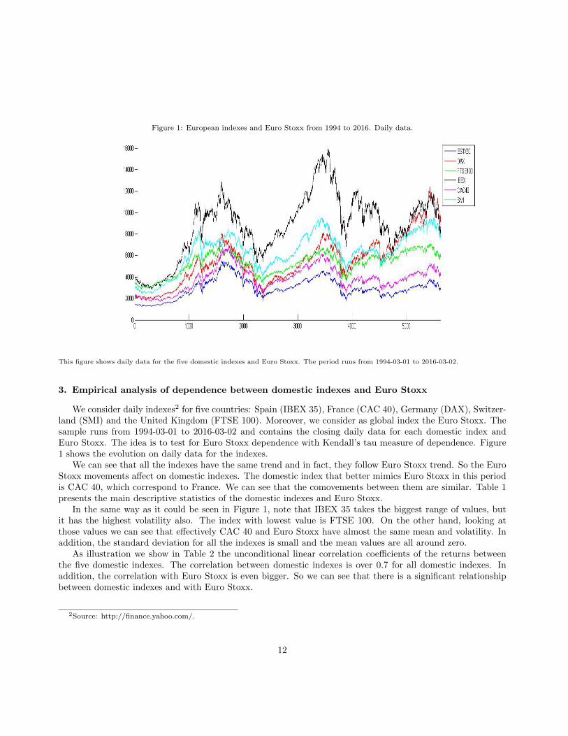
Figure 1: European indexes and Euro Stoxx from 1994 to 2016. Daily data.

This figure shows daily data for the five domestic indexes and Euro Stoxx. The period runs from 1994-03-01 to 2016-03-02.

3. Empirical analysis of dependence between domestic indexes and Euro Stoxx

We consider daily indexes2 for five countries: Spain (IBEX 35), France (CAC 40), Germany (DAX), Switzer-land (SMI) and the United Kingdom (FTSE 100). Moreover, we consider as global index the Euro Stoxx. Thesample runs from 1994-03-01 to 2016-03-02 and contains the closing daily data for each domestic index andEuro Stoxx. The idea is to test for Euro Stoxx dependence with Kendall’s tau measure of dependence. Figure1 shows the evolution on daily data for the indexes.

We can see that all the indexes have the same trend and in fact, they follow Euro Stoxx trend. So the EuroStoxx movements affect on domestic indexes. The domestic index that better mimics Euro Stoxx in this periodis CAC 40, which correspond to France. We can see that the comovements between them are similar. Table 1presents the main descriptive statistics of the domestic indexes and Euro Stoxx.

In the same way as it could be seen in Figure 1, note that IBEX 35 takes the biggest range of values, butit has the highest volatility also. The index with lowest value is FTSE 100. On the other hand, looking atthose values we can see that effectively CAC 40 and Euro Stoxx have almost the same mean and volatility. Inaddition, the standard deviation for all the indexes is small and the mean values are all around zero.

As illustration we show in Table 2 the unconditional linear correlation coefficients of the returns betweenthe five domestic indexes. The correlation between domestic indexes is over 0.7 for all domestic indexes. Inaddition, the correlation with Euro Stoxx is even bigger. So we can see that there is a significant relationshipbetween domestic indexes and with Euro Stoxx.

2Source: http://finance.yahoo.com/.

12

Table 1: Descriptive statistics of daily domestic indexes and Euro Stoxx

Min Max Mean Std.

EUROSTOXX 50 -0.0821 0.1044 0.000138 0.0147

DAX -0.0743 0.1080 0.000273 0.0152

FTSE 100 -0.0926 0.0938 0.000110 0.0119

IBEX 35 -0.0959 0.1348 0.000164 0.0151

CAC 40 -0.0947 0.1060 0.000124 0.0148

SMI -0.0907 0.1079 0.000184 0.0122

This table presents the descriptive statistics for the following daily indexes: EUROSTOXX 50 (Euro Stoxx), DAX (Germany), FTSE 100

(United Kingdom), IBEX 35 (Spain), CAC 40 (France) and SMI(Switzerland).

Table 2: Domestic index returns and Euro Stoxx: unconditional linear correlation coefficients

DAX FTSE 100 IBEX 35 CAC 40 SMI EUROSTOXX

DAX 1 0.790 0.772 0.857 0.763 0.9202

FTSE 100 1 0.767 0.860 0.780 0.8648

IBEX 35 1 0.845 0.725 0.8809

CAC 40 1 0.793 0.9552

SMI 1 0.814

This table presents the unconditional linear correlation coefficients for daily indexes: DAX (Germany), FTSE 100 (United Kingdom), IBEX

35 (Spain), CAC 40 (France) and SMI (Switzerland).

Taking into account the procedure described in Section 1 and in order to show some estimated copulas,we have calculated the conditional copula estimates for several values of Euro Stoxx. The values of EuroStoxx to condition on will be quantiles 0.01, 0.1, 0.25, 0.50, 0.75, 0.9 and 0.99, which are represented byq0.01, q0.1, q0.25, q0.5, q0.75, q0.9 and q0.99 respectively. Figure 2 shows the estimates for DAX and FTSE 100. Itcan be observed that when we condition to tail values there are not many observations to estimate each point;that’s why we obtain a stepped shape. However, the closer is Euro Stoxx value to the mean the more plane thedistribution function is.

We would like to test for Euro Stoxx dependence with Kendall’s tau measure of dependence. To do so, weare going to condition to some values of Euro Stoxx, such as quantile 0.01, 0.1, 0.25, 0.5, 0.75, 0.9 and 0.99(which are represented by q0.01, q0.1, q0.25, q0.5, q0.75, q0.9 and q0.99 respectively). Then, we will try to answerthe following question: Are the measures for the conditioning values equal and the same to the uncoditionalmeasure or not?

So, we suggest the following hypothesis test:

H0 : τ = τq0.01 = τq0.1 = τq0.25 = τq0.5 = τq0.75 = τq0.9 = τq0.99

Ha : τ 6= τi, i = q0.01, q0.1, q0.25, q0.5, q0.75, q0.9, q0.99

If H0 is satisfied, Kendall’s tau coefficient is the same for all conditioning values of Eurostoxx, that is, itmust be equal to the unconditional Kendall’s coefficient. There is no doubt that calculating the unconditionalcoefficient is easier than calculating the conditional one. Note that τn coincides with the estimator defined in(3) when parameters h, g1 and g2 go to infinity. The nonparametric unconditional Kendall’s tau version is givenby

13

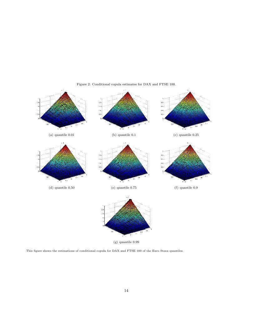
Figure 2: Conditional copula estimates for DAX and FTSE 100.

(a) quantile 0.01 (b) quantile 0.1 (c) quantile 0.25

(d) quantile 0.50 (e) quantile 0.75 (f) quantile 0.9

(g) quantile 0.99

This figure shows the estimations of conditional copula for DAX and FTSE 100 of the Euro Stoxx quantiles.

14

τn = 4n(n−1)

∑ni=1

∑nj=1 I{Y1i < Y1j , Y2i < Y2j} − 1.

In this case, Kendall’s tau could be considered the same, no matter what the conditionant value is. On thecontrary, if the alternative hypothesis is satisfied, it’s not necessary to do the complex procedure of calculatingconditional copulas and it’s enough with the general theory of unconditional copulas. Moreover, given this fact,the relationship between index returns does not depend on Euro Stoxx values.

To decide somehow when the null hypothesis is satisfied we calculate the confidence interval for uncoditionalKendall’s tau,

[τ − στu1−α2 , τ + στu1−α2 ],

where u1−α2 is the corresponding quantile of the standard normal distribution and α ∈ (0, 1) confidencelevel. στ makes reference to the standard deviation of τ . We don’t know the real value, so we will estimate itvia Jackknife estimator.

3.1. Estimator of Kendall’s tau variance.

The jackknife is a resampling technique developed by Quenouille (1949) to estimate the bias of an estimator.Tukey (1958) expanded the use of the procedure to include variance estimation. This procedure is stronglyrelated to an other resampling method such as the bootstrap (i.e., the jackknife is often a linear approximationof the bootstrap), which is the main technique for computational estimation of population parameters. Thejackknife estimation of a parameter is an iterative process.

Let θ be the parameter and T its jackknife estimate. The sample of N observations is a set denoted{X1, · · · , Xn, · · · , XN}. The sample estimate of the parameter θ is a function T = f(X1, · · · , Xn, · · · , XN ) of theobservations in the sample. An estimation of the population parameter obtained removing the n-th observation,called the n-th partial prediction and denoted T−n, is a function T−n = f(X1, · · · , Xn−1, · · · , Xn+1, · · · , XN ).Moreover, T• is obtained as the mean of the partial predictions

T• =∑ni=1 T−i

Hence, the variance of the parameter estimates is denoted

σ2T = n−1

n

∑ni=1(T−i − T•)2

Our parameter is Kendall’s tau, so what we would like to estimate is tau’s variance. Thus, the estimatedvariance will be

σ2τ = n−1

n

∑ni=1(τ−i − τ•)2,

where τ• = 1n

∑ni=1 τ−i .

Instead of doing directly a leave-one-out procedure, we have implemented the procedure leaving out 1, 5,10, 15 and 20 observations. The results obtained were similar and we reached to the same conclusions, so dueto programming efficiency and to getting a representative number of estimations, we are going to leave out 10observations of the sample on the calculation of each Kendall’s tau. This way we have 538 estimated coefficientsto calculate the estimated variance.

In order to see the sensitivity of Kendall’s tau to the bandwidth choice, we consider different values for theh based on the one used to estimate the conditional copula. The value h = 0.0018 considered before impliestaking about the nearest 9 observations to estimate each point. For the values of τ conditioned to quantiles

15

0.01 and 0.99 it is necessary to increase the h value (i.e. we take 3h as we did before when calculating copulas)because there is a small amount of observations on the tails while estimating each point.

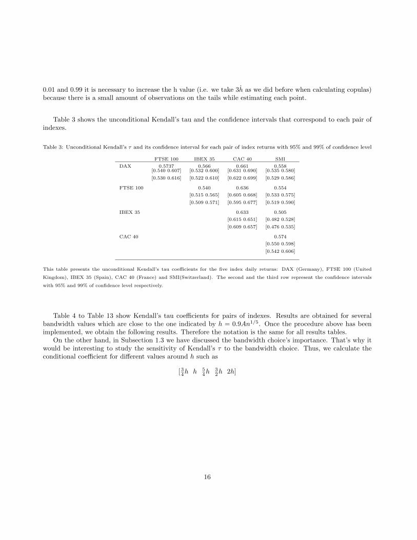
Table 3 shows the unconditional Kendall’s tau and the confidence intervals that correspond to each pair ofindexes.

Table 3: Unconditional Kendall’s τ and its confidence interval for each pair of index returns with 95% and 99% of confidence level

FTSE 100 IBEX 35 CAC 40 SMI

DAX 0.5737 0.566 0.661 0.558[0.540 0.607] [0.532 0.600] [0.631 0.690] [0.535 0.580]

[0.530 0.616] [0.522 0.610] [0.622 0.699] [0.529 0.586]

FTSE 100 0.540 0.636 0.554

[0.515 0.565] [0.605 0.668] [0.533 0.575]

[0.509 0.571] [0.595 0.677] [0.519 0.590]

IBEX 35 0.633 0.505

[0.615 0.651] [0.482 0.528]

[0.609 0.657] [0.476 0.535]

CAC 40 0.574

[0.550 0.598]

[0.542 0.606]

This table presents the unconditional Kendall’s tau coefficients for the five index daily returns: DAX (Germany), FTSE 100 (United

Kingdom), IBEX 35 (Spain), CAC 40 (France) and SMI(Switzerland). The second and the third row represent the confidence intervals

with 95% and 99% of confidence level respectively.

Table 4 to Table 13 show Kendall’s tau coefficients for pairs of indexes. Results are obtained for severalbandwidth values which are close to the one indicated by h = 0.9An1/5. Once the procedure above has beenimplemented, we obtain the following results. Therefore the notation is the same for all results tables.

On the other hand, in Subsection 1.3 we have discussed the bandwidth choice’s importance. That’s why itwould be interesting to study the sensitivity of Kendall’s τ to the bandwidth choice. Thus, we calculate theconditional coefficient for different values around h such as

[ 34h h 5

4h32h 2h]

16

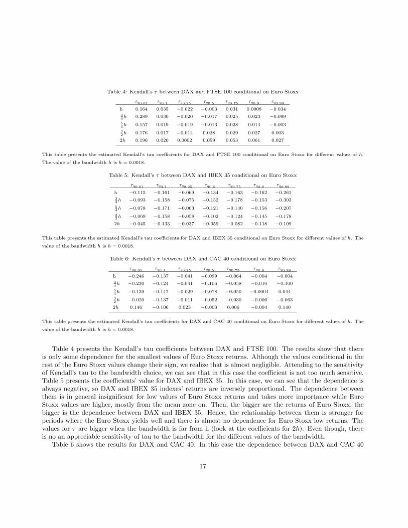
Table 4: Kendall’s τ between DAX and FTSE 100 conditional on Euro Stoxx

τq0.01 τq0.1 τq0.25 τq0.5 τq0.75 τq0.9 τq0.99

h 0.164 0.035 −0.022 −0.003 0.031 0.0008 −0.03434h 0.289 0.030 −0.020 −0.017 0.025 0.023 −0.099

54h 0.157 0.019 −0.019 −0.013 0.028 0.014 −0.003

32h 0.176 0.017 −0.014 0.028 0.029 0.027 0.003

2h 0.196 0.020 0.0002 0.059 0.053 0.061 0.027

This table presents the estimated Kendall’s tau coefficients for DAX and FTSE 100 conditional on Euro Stoxx for different values of h.

The value of the bandwidth h is h = 0.0018.

Table 5: Kendall’s τ between DAX and IBEX 35 conditional on Euro Stoxx

τq0.01 τq0.1 τq0.25 τq0.5 τq0.75 τq0.9 τq0.99

h −0.115 −0.161 −0.069 −0.134 −0.163 −0.162 −0.26134h −0.093 −0.158 −0.075 −0.152 −0.178 −0.153 −0.303

54h −0.078 −0.171 −0.063 −0.121 −0.140 −0.156 −0.207

32h −0.069 −0.158 −0.058 −0.102 −0.124 −0.145 −0.178

2h −0.045 −0.133 −0.037 −0.059 −0.082 −0.118 −0.109

This table presents the estimated Kendall’s tau coefficients for DAX and IBEX 35 conditional on Euro Stoxx for different values of h. The

value of the bandwidth h is h = 0.0018.

Table 6: Kendall’s τ between DAX and CAC 40 conditional on Euro Stoxx

τq0.01 τq0.1 τq0.25 τq0.5 τq0.75 τq0.9 τq0.99

h −0.246 −0.137 −0.041 −0.099 −0.064 −0.004 −0.00434h −0.230 −0.124 −0.041 −0.106 −0.058 −0.010 −0.100

54h −0.139 −0.147 −0.029 −0.078 −0.050 −0.0004 0.044

32h −0.020 −0.137 −0.011 −0.052 −0.030 −0.006 −0.063

2h 0.146 −0.106 0.023 −0.003 0.006 −0.004 0.140

This table presents the estimated Kendall’s tau coefficients for DAX and CAC 40 conditional on Euro Stoxx for different values of h. The


Table 4 presents the Kendall’s tau coefficients between DAX and FTSE 100. The results show that thereis only some dependence for the smallest values of Euro Stoxx returns. Although the values conditional in therest of the Euro Stoxx values change their sign, we realize that is almost negligible. Attending to the sensitivityof Kendall’s tau to the bandwidth choice, we can see that in this case the coefficient is not too much sensitive.Table 5 presents the coefficients’ value for DAX and IBEX 35. In this case, we can see that the dependence isalways negative, so DAX and IBEX 35 indexes’ returns are inversely proportional. The dependence betweenthem is in general insignificant for low values of Euro Stoxx returns and takes more importance while EuroStoxx values are higher, mostly from the mean zone on. Then, the bigger are the returns of Euro Stoxx, thebigger is the dependence between DAX and IBEX 35. Hence, the relationship between them is stronger forperiods where the Euro Stoxx yields well and there is almost no dependence for Euro Stoxx low returns. Thevalues for τ are bigger when the bandwidth is far from h (look at the coefficients for 2h). Even though, thereis no an appreciable sensitivity of tau to the bandwidth for the different values of the bandwidth.

Table 6 shows the results for DAX and CAC 40. In this case the dependence between DAX and CAC 40

17

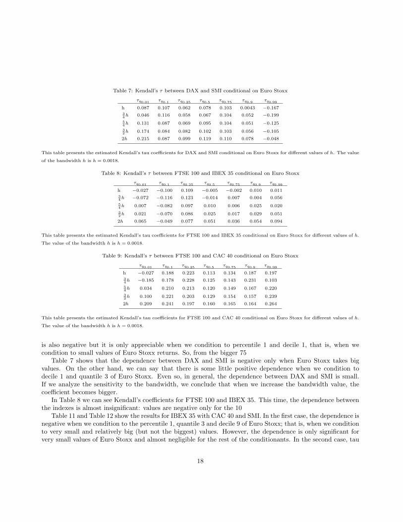
Table 7: Kendall’s τ between DAX and SMI conditional on Euro Stoxx

τq0.01 τq0.1 τq0.25 τq0.5 τq0.75 τq0.9 τq0.99

h 0.087 0.107 0.062 0.078 0.103 0.0043 −0.16734h 0.046 0.116 0.058 0.067 0.104 0.052 −0.199

54h 0.131 0.087 0.069 0.095 0.104 0.051 −0.125

32h 0.174 0.084 0.082 0.102 0.103 0.056 −0.105

2h 0.215 0.087 0.099 0.119 0.110 0.078 −0.048

This table presents the estimated Kendall’s tau coefficients for DAX and SMI conditional on Euro Stoxx for different values of h. The value

of the bandwidth h is h = 0.0018.

Table 8: Kendall’s τ between FTSE 100 and IBEX 35 conditional on Euro Stoxx

τq0.01 τq0.1 τq0.25 τq0.5 τq0.75 τq0.9 τq0.99

h −0.027 −0.100 0.109 −0.005 −0.002 0.010 0.01134h −0.072 −0.116 0.123 −0.014 0.007 0.004 0.056

54h 0.007 −0.082 0.097 0.010 0.006 0.025 0.020

32h 0.021 −0.070 0.086 0.025 0.017 0.029 0.051

2h 0.065 −0.049 0.077 0.051 0.036 0.054 0.094

This table presents the estimated Kendall’s tau coefficients for FTSE 100 and IBEX 35 conditional on Euro Stoxx for different values of h.


Table 9: Kendall’s τ between FTSE 100 and CAC 40 conditional on Euro Stoxx

τq0.01 τq0.1 τq0.25 τq0.5 τq0.75 τq0.9 τq0.99

h −0.027 0.188 0.223 0.113 0.134 0.187 0.19734h −0.185 0.178 0.228 0.125 0.143 0.231 0.103

54h 0.034 0.210 0.213 0.120 0.149 0.167 0.220

32h 0.100 0.221 0.203 0.129 0.154 0.157 0.239

2h 0.209 0.241 0.197 0.160 0.165 0.164 0.264

This table presents the estimated Kendall’s tau coefficients for FTSE 100 and CAC 40 conditional on Euro Stoxx for different values of h.


is also negative but it is only appreciable when we condition to percentile 1 and decile 1, that is, when wecondition to small values of Euro Stoxx returns. So, from the bigger 75

Table 7 shows that the dependence between DAX and SMI is negative only when Euro Stoxx takes bigvalues. On the other hand, we can say that there is some little positive dependence when we condition todecile 1 and quantile 3 of Euro Stoxx. Even so, in general, the dependence between DAX and SMI is small.If we analyze the sensitivity to the bandwidth, we conclude that when we increase the bandwidth value, thecoefficient becomes bigger.

In Table 8 we can see Kendall’s coefficients for FTSE 100 and IBEX 35. This time, the dependence betweenthe indexes is almost insignificant: values are negative only for the 10

Table 11 and Table 12 show the results for IBEX 35 with CAC 40 and SMI. In the first case, the dependence isnegative when we condition to the percentile 1, quantile 3 and decile 9 of Euro Stoxx; that is, when we conditionto very small and relatively big (but not the biggest) values. However, the dependence is only significant forvery small values of Euro Stoxx and almost negligible for the rest of the conditionants. In the second case, tau

18

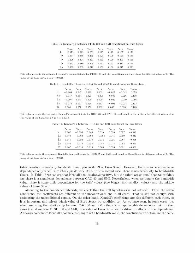
Table 10: Kendall’s τ between FTSE 100 and SMI conditional on Euro Stoxx

τq0.01 τq0.1 τq0.25 τq0.5 τq0.75 τq0.9 τq0.99

h 0.179 0.319 0.252 0.127 0.115 0.187 0.17634h 0.137 0.348 0.262 0.123 0.109 0.173 0.185

54h 0.228 0.304 0.243 0.132 0.120 0.201 0.165

32h 0.261 0.289 0.228 0.141 0.122 0.213 0.175

2h 0.303 0.265 0.219 0.158 0.138 0.217 0.221

This table presents the estimated Kendall’s tau coefficients for FTSE 100 and SMI conditional on Euro Stoxx for different values of h. The


Table 11: Kendall’s τ between IBEX 35 and CAC 40 conditional on Euro Stoxx

τq0.01 τq0.1 τq0.25 τq0.5 τq0.75 τq0.9 τq0.99

h −0.203 0.047 0.023 0.002 −0.027 −0.042 0.07934h −0.317 0.054 0.023 −0.005 −0.035 −0.026 0.118

54h −0.097 0.044 0.025 0.020 −0.022 −0.039 0.086

32h −0.038 0.043 0.030 0.041 −0.001 −0.014 0.113

2h 0.050 0.055 0.058 0.082 0.033 0.023 0.165

This table presents the estimated Kendall’s tau coefficients for IBEX 35 and CAC 40 conditional on Euro Stoxx for different values of h.


Table 12: Kendall’s τ between IBEX 35 and SMI conditional on Euro Stoxx

τq0.01 τq0.1 τq0.25 τq0.5 τq0.75 τq0.9 τq0.99

h 0.162 −0.036 0.044 0.019 0.033 0.057 −0.04234h 0.170 −0.062 0.060 −0.004 0.045 0.029 −0.012

54h 0.175 −0.024 0.038 0.034 0.021 0.067 −0.058

32h 0.156 −0.018 0.028 0.045 0.018 0.083 −0.041

2h 0.167 −0.015 0.018 0.068 0.023 0.091 −0.008

This table presents the estimated Kendall’s tau coefficients for IBEX 35 and SMI conditional on Euro Stoxx for different values of h. The


takes negative values only for decile 1 and percentile 99 of Euro Stoxx. However, there is some appreciabledependence only when Euro Stoxx yields very little. In this second case, there is not sensitivity to bandwidthchoice. In Table 13 we can see that Kendall’s tau is always positive, but the values are so small that we couldn’tsay there is a significant dependence between CAC 40 and SMI. Nevertheless, when we double the bandwithvalue, there is some little dependence for the tails’ values (the biggest and smallest values) and the middlevalues of Euro Stoxx.

Attending to the confidence intervals, we check that the null hypothesis is not satisfied. Thus, the sevenconditional tau coefficients are different to the unconditional one in all cases. That is, it’s not enough withestimating the unconditional copula. On the other hand, Kendall’s coefficients are also different each other, soit is important and affects which value of Euro Stoxx we condition to. As we have seen, in some cases (i.e.when analyzing the relationship between CAC 40 and SMI) there is no appreciable dependence but in othercases (i.e. if we take FTSE 100 and SMI), the value of Euro Stoxx we condition to affects to the dependence.Although sometimes Kendall’s coefficient changes with bandwidth value, the conclusions we obtain are the same

19

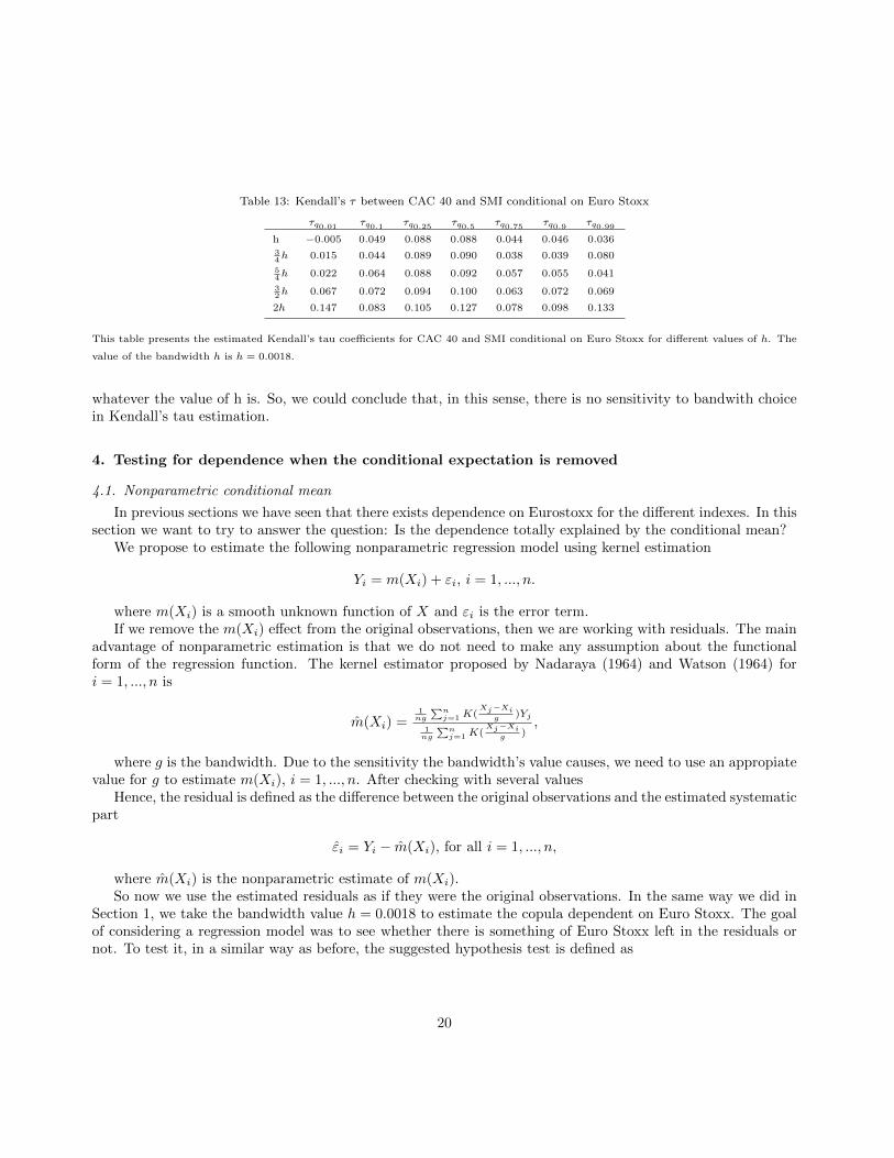
Table 13: Kendall’s τ between CAC 40 and SMI conditional on Euro Stoxx

τq0.01 τq0.1 τq0.25 τq0.5 τq0.75 τq0.9 τq0.99

h −0.005 0.049 0.088 0.088 0.044 0.046 0.03634h 0.015 0.044 0.089 0.090 0.038 0.039 0.080

54h 0.022 0.064 0.088 0.092 0.057 0.055 0.041

32h 0.067 0.072 0.094 0.100 0.063 0.072 0.069

2h 0.147 0.083 0.105 0.127 0.078 0.098 0.133

This table presents the estimated Kendall’s tau coefficients for CAC 40 and SMI conditional on Euro Stoxx for different values of h. The


whatever the value of h is. So, we could conclude that, in this sense, there is no sensitivity to bandwith choicein Kendall’s tau estimation.

4. Testing for dependence when the conditional expectation is removed

4.1. Nonparametric conditional mean

In previous sections we have seen that there exists dependence on Eurostoxx for the different indexes. In thissection we want to try to answer the question: Is the dependence totally explained by the conditional mean?

We propose to estimate the following nonparametric regression model using kernel estimation

Yi = m(Xi) + εi, i = 1, ..., n.

where m(Xi) is a smooth unknown function of X and εi is the error term.If we remove the m(Xi) effect from the original observations, then we are working with residuals. The main

advantage of nonparametric estimation is that we do not need to make any assumption about the functionalform of the regression function. The kernel estimator proposed by Nadaraya (1964) and Watson (1964) fori = 1, ..., n is

m(Xi) =1ng

∑nj=1K(

Xj−Xig )Yj

1ng

∑nj=1K(

Xj−Xig )

,

where g is the bandwidth. Due to the sensitivity the bandwidth’s value causes, we need to use an appropiatevalue for g to estimate m(Xi), i = 1, ..., n. After checking with several values

Hence, the residual is defined as the difference between the original observations and the estimated systematicpart

εi = Yi − m(Xi), for all i = 1, ..., n,

where m(Xi) is the nonparametric estimate of m(Xi).So now we use the estimated residuals as if they were the original observations. In the same way we did in

Section 1, we take the bandwidth value h = 0.0018 to estimate the copula dependent on Euro Stoxx. The goalof considering a regression model was to see whether there is something of Euro Stoxx left in the residuals ornot. To test it, in a similar way as before, the suggested hypothesis test is defined as

20

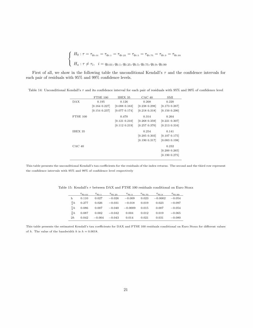
H0 : τ = τq0.01 = τq0.1 = τq0.25 = τq0.5 = τq0.75 = τq0.9 = τq0.99

Ha : τ 6= τi, i = q0.01, q0.1, q0.25, q0.5, q0.75, q0.9, q0.99

First of all, we show in the following table the unconditional Kendall’s τ and the confidence intervals foreach pair of residuals with 95% and 99% confidence levels.

Table 14: Unconditional Kendall’s τ and its confidence interval for each pair of residuals with 95% and 99% of confidence level


DAX 0.195 0.126 0.268 0.220

[0.164 0.227] [0.088 0.163] [0.238 0.298] [0.173 0.267]

[0.154 0.237] [0.077 0.174] [0.218 0.318] [0.150 0.290]

FTSE 100 0.470 0.314 0.264

[0.121 0.210] [0.268 0.359] [0.221 0.307]

[0.112 0.219] [0.257 0.370] [0.213 0.316]

IBEX 35 0.254 0.141

[0.205 0.303] [0.107 0.175]

[0.190 0.317] [0.083 0.198]

CAC 40 0.232

[0.200 0.265]

[0.190 0.275]

This table presents the unconditional Kendall’s tau coefficients for the residuals of the index returns. The second and the third row represent

the confidence intervals with 95% and 99% of confidence level respectively

Table 15: Kendall’s τ between DAX and FTSE 100 residuals conditional on Euro Stoxx

τq0.01 τq0.1 τq0.25 τq0.5 τq0.75 τq0.9 τq0.99

h 0.110 0.027 −0.026 −0.009 0.023 −0.0002 −0.05434h 0.277 0.026 −0.031 −0.018 0.019 0.023 −0.097

54h 0.086 0.007 −0.040 −0.0009 0.015 0.007 −0.054

32h 0.087 0.002 −0.042 0.004 0.012 0.019 −0.065

2h 0.042 −0.004 −0.043 0.014 0.021 0.031 −0.080

This table presents the estimated Kendall’s tau coefficients for DAX and FTSE 100 residuals conditional on Euro Stoxx for different values

of h. The value of the bandwidth h is h = 0.0018.

21

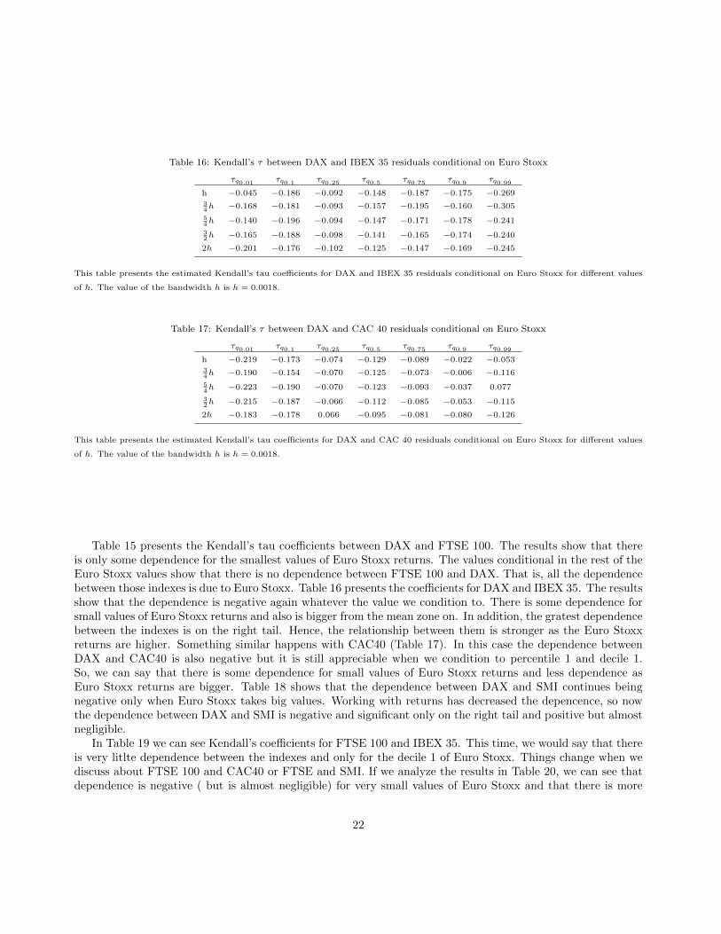
Table 16: Kendall’s τ between DAX and IBEX 35 residuals conditional on Euro Stoxx

τq0.01 τq0.1 τq0.25 τq0.5 τq0.75 τq0.9 τq0.99

h −0.045 −0.186 −0.092 −0.148 −0.187 −0.175 −0.26934h −0.168 −0.181 −0.093 −0.157 −0.195 −0.160 −0.305

54h −0.140 −0.196 −0.094 −0.147 −0.171 −0.178 −0.241

32h −0.165 −0.188 −0.098 −0.141 −0.165 −0.174 −0.240

2h −0.201 −0.176 −0.102 −0.125 −0.147 −0.169 −0.245

This table presents the estimated Kendall’s tau coefficients for DAX and IBEX 35 residuals conditional on Euro Stoxx for different values


Table 17: Kendall’s τ between DAX and CAC 40 residuals conditional on Euro Stoxx

τq0.01 τq0.1 τq0.25 τq0.5 τq0.75 τq0.9 τq0.99

h −0.219 −0.173 −0.074 −0.129 −0.089 −0.022 −0.05334h −0.190 −0.154 −0.070 −0.125 −0.073 −0.006 −0.116

54h −0.223 −0.190 −0.070 −0.123 −0.093 −0.037 0.077

32h −0.215 −0.187 −0.066 −0.112 −0.085 −0.053 −0.115

2h −0.183 −0.178 0.066 −0.095 −0.081 −0.080 −0.126

This table presents the estimated Kendall’s tau coefficients for DAX and CAC 40 residuals conditional on Euro Stoxx for different values


Table 15 presents the Kendall’s tau coefficients between DAX and FTSE 100. The results show that thereis only some dependence for the smallest values of Euro Stoxx returns. The values conditional in the rest of theEuro Stoxx values show that there is no dependence between FTSE 100 and DAX. That is, all the dependencebetween those indexes is due to Euro Stoxx. Table 16 presents the coefficients for DAX and IBEX 35. The resultsshow that the dependence is negative again whatever the value we condition to. There is some dependence forsmall values of Euro Stoxx returns and also is bigger from the mean zone on. In addition, the gratest dependencebetween the indexes is on the right tail. Hence, the relationship between them is stronger as the Euro Stoxxreturns are higher. Something similar happens with CAC40 (Table 17). In this case the dependence betweenDAX and CAC40 is also negative but it is still appreciable when we condition to percentile 1 and decile 1.So, we can say that there is some dependence for small values of Euro Stoxx returns and less dependence asEuro Stoxx returns are bigger. Table 18 shows that the dependence between DAX and SMI continues beingnegative only when Euro Stoxx takes big values. Working with returns has decreased the depencence, so nowthe dependence between DAX and SMI is negative and significant only on the right tail and positive but almostnegligible.

In Table 19 we can see Kendall’s coefficients for FTSE 100 and IBEX 35. This time, we would say that thereis very litlte dependence between the indexes and only for the decile 1 of Euro Stoxx. Things change when wediscuss about FTSE 100 and CAC40 or FTSE and SMI. If we analyze the results in Table 20, we can see thatdependence is negative ( but is almost negligible) for very small values of Euro Stoxx and that there is more

22

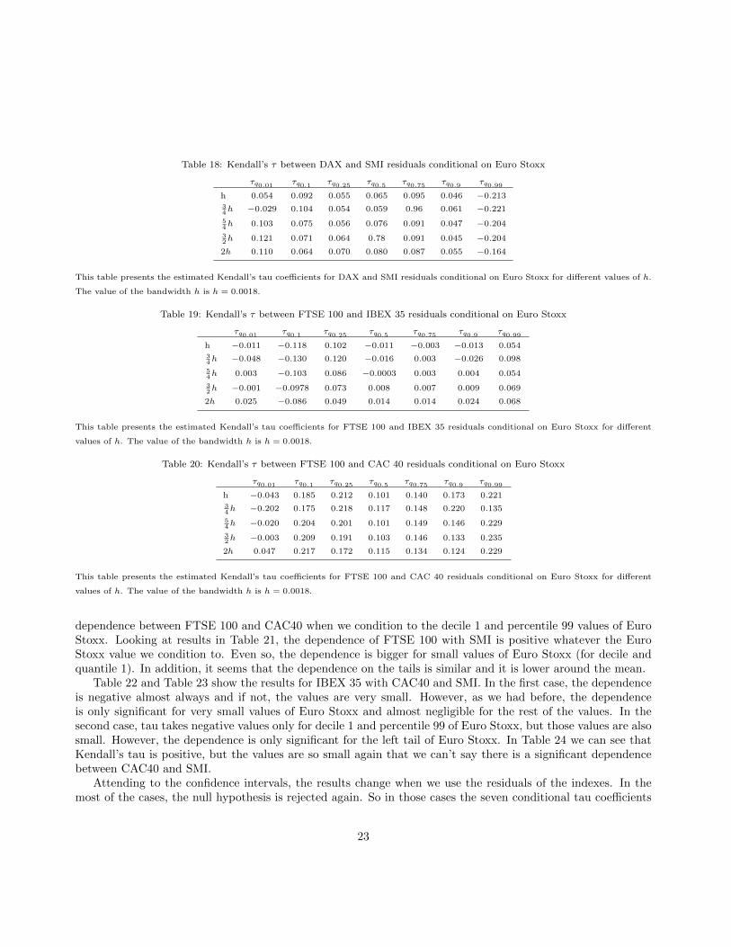
Table 18: Kendall’s τ between DAX and SMI residuals conditional on Euro Stoxx

τq0.01 τq0.1 τq0.25 τq0.5 τq0.75 τq0.9 τq0.99

h 0.054 0.092 0.055 0.065 0.095 0.046 −0.21334h −0.029 0.104 0.054 0.059 0.96 0.061 −0.221

54h 0.103 0.075 0.056 0.076 0.091 0.047 −0.204

32h 0.121 0.071 0.064 0.78 0.091 0.045 −0.204

2h 0.110 0.064 0.070 0.080 0.087 0.055 −0.164

This table presents the estimated Kendall’s tau coefficients for DAX and SMI residuals conditional on Euro Stoxx for different values of h.


Table 19: Kendall’s τ between FTSE 100 and IBEX 35 residuals conditional on Euro Stoxx

τq0.01 τq0.1 τq0.25 τq0.5 τq0.75 τq0.9 τq0.99

h −0.011 −0.118 0.102 −0.011 −0.003 −0.013 0.05434h −0.048 −0.130 0.120 −0.016 0.003 −0.026 0.098

54h 0.003 −0.103 0.086 −0.0003 0.003 0.004 0.054

32h −0.001 −0.0978 0.073 0.008 0.007 0.009 0.069

2h 0.025 −0.086 0.049 0.014 0.014 0.024 0.068

This table presents the estimated Kendall’s tau coefficients for FTSE 100 and IBEX 35 residuals conditional on Euro Stoxx for different

values of h. The value of the bandwidth h is h = 0.0018.

Table 20: Kendall’s τ between FTSE 100 and CAC 40 residuals conditional on Euro Stoxx

τq0.01 τq0.1 τq0.25 τq0.5 τq0.75 τq0.9 τq0.99

h −0.043 0.185 0.212 0.101 0.140 0.173 0.22134h −0.202 0.175 0.218 0.117 0.148 0.220 0.135

54h −0.020 0.204 0.201 0.101 0.149 0.146 0.229

32h −0.003 0.209 0.191 0.103 0.146 0.133 0.235

2h 0.047 0.217 0.172 0.115 0.134 0.124 0.229

This table presents the estimated Kendall’s tau coefficients for FTSE 100 and CAC 40 residuals conditional on Euro Stoxx for different


dependence between FTSE 100 and CAC40 when we condition to the decile 1 and percentile 99 values of EuroStoxx. Looking at results in Table 21, the dependence of FTSE 100 with SMI is positive whatever the EuroStoxx value we condition to. Even so, the dependence is bigger for small values of Euro Stoxx (for decile andquantile 1). In addition, it seems that the dependence on the tails is similar and it is lower around the mean.

Table 22 and Table 23 show the results for IBEX 35 with CAC40 and SMI. In the first case, the dependenceis negative almost always and if not, the values are very small. However, as we had before, the dependenceis only significant for very small values of Euro Stoxx and almost negligible for the rest of the values. In thesecond case, tau takes negative values only for decile 1 and percentile 99 of Euro Stoxx, but those values are alsosmall. However, the dependence is only significant for the left tail of Euro Stoxx. In Table 24 we can see thatKendall’s tau is positive, but the values are so small again that we can’t say there is a significant dependencebetween CAC40 and SMI.

Attending to the confidence intervals, the results change when we use the residuals of the indexes. In themost of the cases, the null hypothesis is rejected again. So in those cases the seven conditional tau coefficients

23

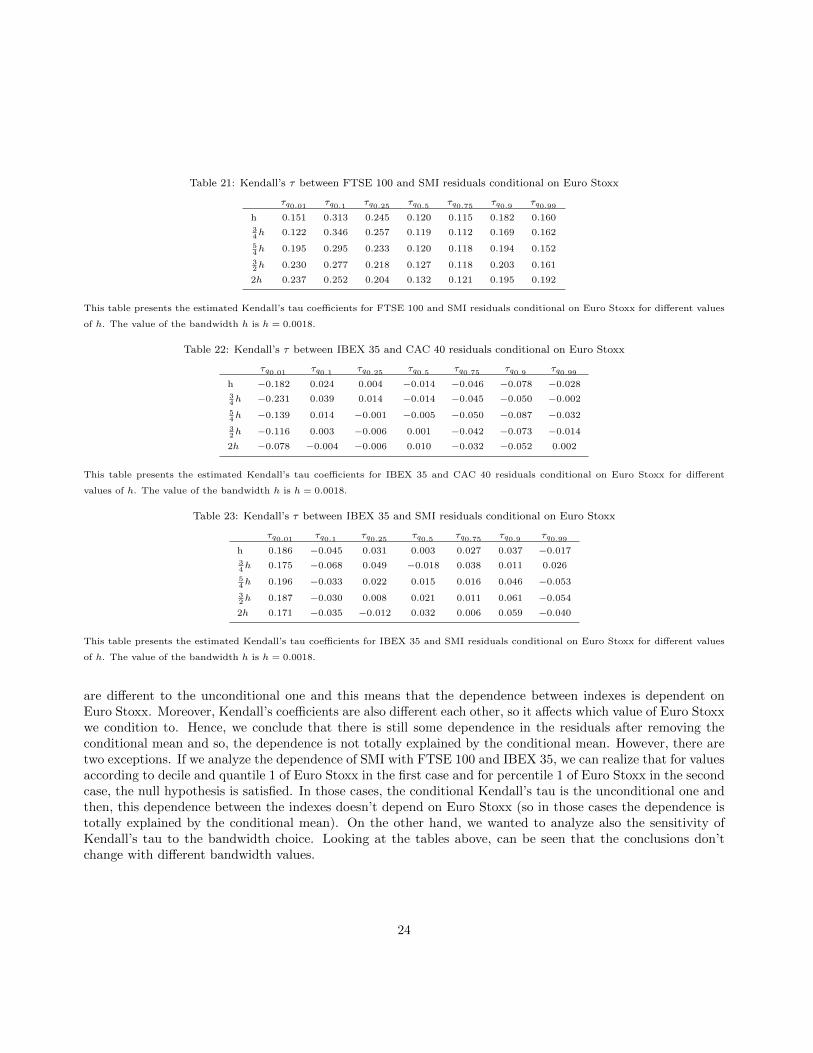
Table 21: Kendall’s τ between FTSE 100 and SMI residuals conditional on Euro Stoxx

τq0.01 τq0.1 τq0.25 τq0.5 τq0.75 τq0.9 τq0.99

h 0.151 0.313 0.245 0.120 0.115 0.182 0.16034h 0.122 0.346 0.257 0.119 0.112 0.169 0.162

54h 0.195 0.295 0.233 0.120 0.118 0.194 0.152

32h 0.230 0.277 0.218 0.127 0.118 0.203 0.161

2h 0.237 0.252 0.204 0.132 0.121 0.195 0.192

This table presents the estimated Kendall’s tau coefficients for FTSE 100 and SMI residuals conditional on Euro Stoxx for different values


Table 22: Kendall’s τ between IBEX 35 and CAC 40 residuals conditional on Euro Stoxx

τq0.01 τq0.1 τq0.25 τq0.5 τq0.75 τq0.9 τq0.99

h −0.182 0.024 0.004 −0.014 −0.046 −0.078 −0.02834h −0.231 0.039 0.014 −0.014 −0.045 −0.050 −0.002

54h −0.139 0.014 −0.001 −0.005 −0.050 −0.087 −0.032

32h −0.116 0.003 −0.006 0.001 −0.042 −0.073 −0.014

2h −0.078 −0.004 −0.006 0.010 −0.032 −0.052 0.002

This table presents the estimated Kendall’s tau coefficients for IBEX 35 and CAC 40 residuals conditional on Euro Stoxx for different


Table 23: Kendall’s τ between IBEX 35 and SMI residuals conditional on Euro Stoxx

τq0.01 τq0.1 τq0.25 τq0.5 τq0.75 τq0.9 τq0.99

h 0.186 −0.045 0.031 0.003 0.027 0.037 −0.01734h 0.175 −0.068 0.049 −0.018 0.038 0.011 0.026

54h 0.196 −0.033 0.022 0.015 0.016 0.046 −0.053

32h 0.187 −0.030 0.008 0.021 0.011 0.061 −0.054

2h 0.171 −0.035 −0.012 0.032 0.006 0.059 −0.040

This table presents the estimated Kendall’s tau coefficients for IBEX 35 and SMI residuals conditional on Euro Stoxx for different values


are different to the unconditional one and this means that the dependence between indexes is dependent onEuro Stoxx. Moreover, Kendall’s coefficients are also different each other, so it affects which value of Euro Stoxxwe condition to. Hence, we conclude that there is still some dependence in the residuals after removing theconditional mean and so, the dependence is not totally explained by the conditional mean. However, there aretwo exceptions. If we analyze the dependence of SMI with FTSE 100 and IBEX 35, we can realize that for valuesaccording to decile and quantile 1 of Euro Stoxx in the first case and for percentile 1 of Euro Stoxx in the secondcase, the null hypothesis is satisfied. In those cases, the conditional Kendall’s tau is the unconditional one andthen, this dependence between the indexes doesn’t depend on Euro Stoxx (so in those cases the dependence istotally explained by the conditional mean). On the other hand, we wanted to analyze also the sensitivity ofKendall’s tau to the bandwidth choice. Looking at the tables above, can be seen that the conclusions don’tchange with different bandwidth values.

24

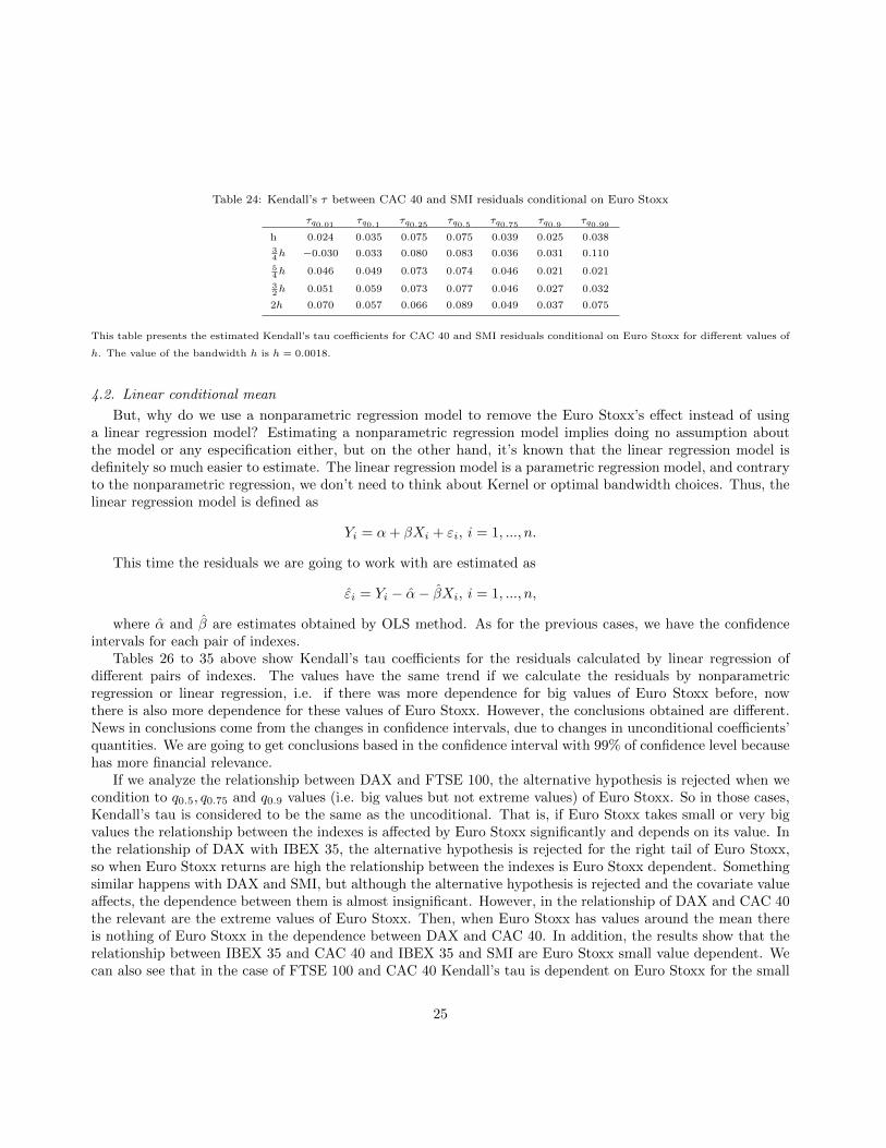
Table 24: Kendall’s τ between CAC 40 and SMI residuals conditional on Euro Stoxx

τq0.01 τq0.1 τq0.25 τq0.5 τq0.75 τq0.9 τq0.99

h 0.024 0.035 0.075 0.075 0.039 0.025 0.03834h −0.030 0.033 0.080 0.083 0.036 0.031 0.110

54h 0.046 0.049 0.073 0.074 0.046 0.021 0.021

32h 0.051 0.059 0.073 0.077 0.046 0.027 0.032

2h 0.070 0.057 0.066 0.089 0.049 0.037 0.075

This table presents the estimated Kendall’s tau coefficients for CAC 40 and SMI residuals conditional on Euro Stoxx for different values of

h. The value of the bandwidth h is h = 0.0018.

4.2. Linear conditional mean

But, why do we use a nonparametric regression model to remove the Euro Stoxx’s effect instead of usinga linear regression model? Estimating a nonparametric regression model implies doing no assumption aboutthe model or any especification either, but on the other hand, it’s known that the linear regression model isdefinitely so much easier to estimate. The linear regression model is a parametric regression model, and contraryto the nonparametric regression, we don’t need to think about Kernel or optimal bandwidth choices. Thus, thelinear regression model is defined as

Yi = α+ βXi + εi, i = 1, ..., n.

This time the residuals we are going to work with are estimated as

εi = Yi − α− βXi, i = 1, ..., n,

where α and β are estimates obtained by OLS method. As for the previous cases, we have the confidenceintervals for each pair of indexes.

Tables 26 to 35 above show Kendall’s tau coefficients for the residuals calculated by linear regression ofdifferent pairs of indexes. The values have the same trend if we calculate the residuals by nonparametricregression or linear regression, i.e. if there was more dependence for big values of Euro Stoxx before, nowthere is also more dependence for these values of Euro Stoxx. However, the conclusions obtained are different.News in conclusions come from the changes in confidence intervals, due to changes in unconditional coefficients’quantities. We are going to get conclusions based in the confidence interval with 99% of confidence level becausehas more financial relevance.

If we analyze the relationship between DAX and FTSE 100, the alternative hypothesis is rejected when wecondition to q0.5, q0.75 and q0.9 values (i.e. big values but not extreme values) of Euro Stoxx. So in those cases,Kendall’s tau is considered to be the same as the uncoditional. That is, if Euro Stoxx takes small or very bigvalues the relationship between the indexes is affected by Euro Stoxx significantly and depends on its value. Inthe relationship of DAX with IBEX 35, the alternative hypothesis is rejected for the right tail of Euro Stoxx,so when Euro Stoxx returns are high the relationship between the indexes is Euro Stoxx dependent. Somethingsimilar happens with DAX and SMI, but although the alternative hypothesis is rejected and the covariate valueaffects, the dependence between them is almost insignificant. However, in the relationship of DAX and CAC 40the relevant are the extreme values of Euro Stoxx. Then, when Euro Stoxx has values around the mean thereis nothing of Euro Stoxx in the dependence between DAX and CAC 40. In addition, the results show that therelationship between IBEX 35 and CAC 40 and IBEX 35 and SMI are Euro Stoxx small value dependent. Wecan also see that in the case of FTSE 100 and CAC 40 Kendall’s tau is dependent on Euro Stoxx for the small

25

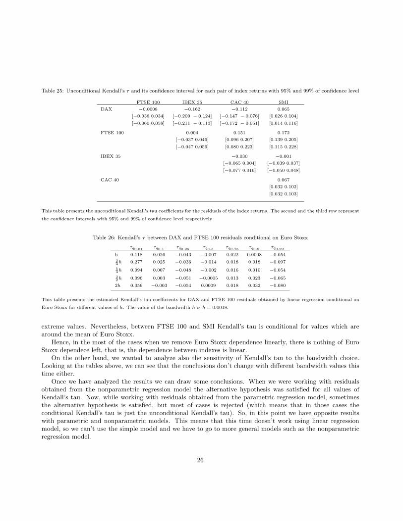
Table 25: Unconditional Kendall’s τ and its confidence interval for each pair of index returns with 95% and 99% of confidence level


DAX −0.0008 −0.162 −0.112 0.065

[−0.036 0.034] [−0.200 − 0.124] [−0.147 − 0.076] [0.026 0.104]

[−0.060 0.058] [−0.211 − 0.113] [−0.172 − 0.051] [0.014 0.116]

FTSE 100 0.004 0.151 0.172

[−0.037 0.046] [0.096 0.207] [0.139 0.205]

[−0.047 0.056] [0.080 0.223] [0.115 0.228]

IBEX 35 −0.030 −0.001

[−0.065 0.004] [−0.039 0.037]

[−0.077 0.016] [−0.050 0.048]

CAC 40 0.067

[0.032 0.102]

[0.032 0.103]

This table presents the unconditional Kendall’s tau coefficients for the residuals of the index returns. The second and the third row represent

the confidence intervals with 95% and 99% of confidence level respectively

Table 26: Kendall’s τ between DAX and FTSE 100 residuals conditional on Euro Stoxx

τq0.01 τq0.1 τq0.25 τq0.5 τq0.75 τq0.9 τq0.99

h 0.118 0.026 −0.043 −0.007 0.022 0.0008 −0.05434h 0.277 0.025 −0.036 −0.014 0.018 0.018 −0.097

54h 0.094 0.007 −0.048 −0.002 0.016 0.010 −0.054

32h 0.096 0.003 −0.051 −0.0005 0.013 0.023 −0.065

2h 0.056 −0.003 −0.054 0.0009 0.018 0.032 −0.080

This table presents the estimated Kendall’s tau coefficients for DAX and FTSE 100 residuals obtained by linear regression conditional on

Euro Stoxx for different values of h. The value of the bandwidth h is h = 0.0018.

extreme values. Nevertheless, between FTSE 100 and SMI Kendall’s tau is conditional for values which arearound the mean of Euro Stoxx.

Hence, in the most of the cases when we remove Euro Stoxx dependence linearly, there is nothing of EuroStoxx dependece left, that is, the dependence between indexes is linear.

On the other hand, we wanted to analyze also the sensitivity of Kendall’s tau to the bandwidth choice.Looking at the tables above, we can see that the conclusions don’t change with different bandwidth values thistime either.

Once we have analyzed the results we can draw some conclusions. When we were working with residualsobtained from the nonparametric regression model the alternative hypothesis was satisfied for all values ofKendall’s tau. Now, while working with residuals obtained from the parametric regression model, sometimesthe alternative hypothesis is satisfied, but most of cases is rejected (which means that in those cases theconditional Kendall’s tau is just the unconditional Kendall’s tau). So, in this point we have opposite resultswith parametric and nonparametric models. This means that this time doesn’t work using linear regressionmodel, so we can’t use the simple model and we have to go to more general models such as the nonparametricregression model.

26

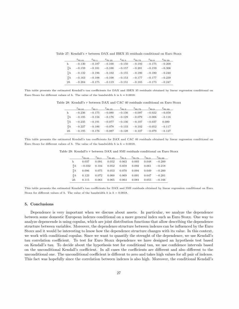
Table 27: Kendall’s τ between DAX and IBEX 35 residuals conditional on Euro Stoxx

τq0.01 τq0.1 τq0.25 τq0.5 τq0.75 τq0.9 τq0.99

h −0.130 −0.187 −0.100 −0.150 −0.193 −0.175 −0.26834h −0.159 −0.181 −0.100 −0.157 −0.201 −0.159 −0.306

54h −0.132 −0.196 −0.102 −0.155 −0.180 −0.180 −0.240

32h −0.163 −0.188 −0.108 −0.153 −0.177 −0.177 −0.239

2h −0.204 −0.175 −0.119 −0.151 −0.165 −0.173 −0.247

This table presents the estimated Kendall’s tau coefficients for DAX and IBEX 35 residuals obtained by linear regression conditional on


Table 28: Kendall’s τ between DAX and CAC 40 residuals conditional on Euro Stoxx

τq0.01 τq0.1 τq0.25 τq0.5 τq0.75 τq0.9 τq0.99

h −0.236 −0.175 −0.080 −0.136 −0.097 −0.022 −0.05834h −0.195 −0.156 −0.176 −0.129 −0.079 −0.006 −0.116

54h −0.235 −0.191 −0.077 −0.136 −0.107 −0.037 0.080

32h −0.227 −0.186 −0.078 −0.133 −0.102 −0.052 −0.117

2h −0.195 −0.176 −0.087 −0.128 −0.107 −0.079 −0.127

This table presents the estimated Kendall’s tau coefficients for DAX and CAC 40 residuals obtained by linear regression conditional on


Table 29: Kendall’s τ between DAX and SMI residuals conditional on Euro Stoxx

τq0.01 τq0.1 τq0.25 τq0.5 τq0.75 τq0.9 τq0.99

h 0.037 0.091 0.052 0.063 0.093 0.048 −0.20934h −0.032 0.104 0.052 0.059 0.092 0.061 −0.218

54h 0.096 0.075 0.053 0.070 0.094 0.049 −0.200

32h 0.123 0.072 0.060 0.069 0.091 0.047 −0.201

2h 0.115 0.064 0.065 0.064 0.084 0.055 −0.166

This table presents the estimated Kendall’s tau coefficients for DAX and SMI residuals obtained by linear regression conditional on Euro

Stoxx for different values of h. The value of the bandwidth h is h = 0.0018.

5. Conclusions

Dependence is very important when we discuss about assets. In particular, we analyze the dependencebetween some domestic European indexes conditional on a more general index such as Euro Stoxx. One way toanalyze depencende is using copulas, which are joint distribution functions that allow describing the dependencestructure between variables. Moreover, the dependence structure between indexes can be influenced by the EuroStoxx and it would be interesting to know how the dependence structure changes with its value. In this context,we work with conditional copulas. Since we want to quantify the strenght of the dependence, we use Kendall’stau correlation coefficient. To test for Euro Stoxx dependence we have designed an hypothesis test basedon Kendall’s tau. To decide about the hypothesis test for conditional tau, we use confidence intervals basedon the unconditional Kendall’s coefficient. In all cases the coefficients are different and also different to theunconditional one. The unconditional coefficient is different to zero and takes high values for all pair of indexes.This fact was hopefully since the correlation between indexes is also high. Moreover, the conditional Kendall’s

27

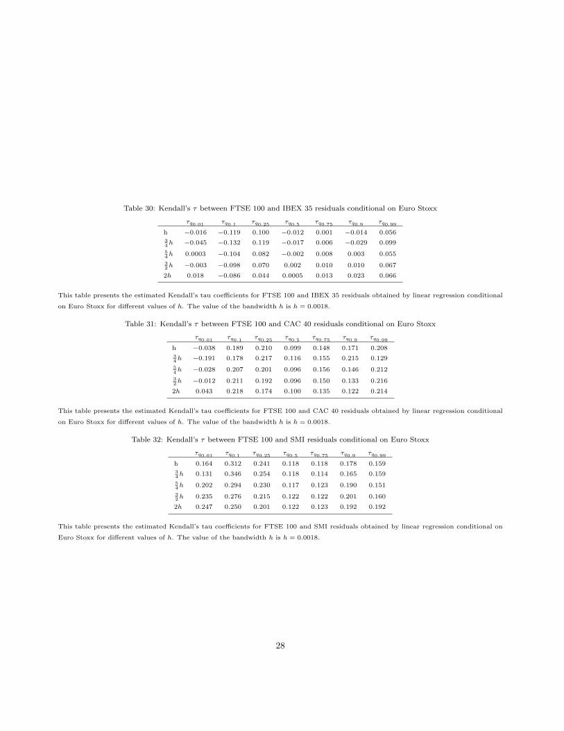
Table 30: Kendall’s τ between FTSE 100 and IBEX 35 residuals conditional on Euro Stoxx

τq0.01 τq0.1 τq0.25 τq0.5 τq0.75 τq0.9 τq0.99

h −0.016 −0.119 0.100 −0.012 0.001 −0.014 0.05634h −0.045 −0.132 0.119 −0.017 0.006 −0.029 0.099

54h 0.0003 −0.104 0.082 −0.002 0.008 0.003 0.055

32h −0.003 −0.098 0.070 0.002 0.010 0.010 0.067

2h 0.018 −0.086 0.044 0.0005 0.013 0.023 0.066

This table presents the estimated Kendall’s tau coefficients for FTSE 100 and IBEX 35 residuals obtained by linear regression conditional

on Euro Stoxx for different values of h. The value of the bandwidth h is h = 0.0018.

Table 31: Kendall’s τ between FTSE 100 and CAC 40 residuals conditional on Euro Stoxx

τq0.01 τq0.1 τq0.25 τq0.5 τq0.75 τq0.9 τq0.99

h −0.038 0.189 0.210 0.099 0.148 0.171 0.20834h −0.191 0.178 0.217 0.116 0.155 0.215 0.129

54h −0.028 0.207 0.201 0.096 0.156 0.146 0.212

32h −0.012 0.211 0.192 0.096 0.150 0.133 0.216

2h 0.043 0.218 0.174 0.100 0.135 0.122 0.214

This table presents the estimated Kendall’s tau coefficients for FTSE 100 and CAC 40 residuals obtained by linear regression conditional

on Euro Stoxx for different values of h. The value of the bandwidth h is h = 0.0018.

Table 32: Kendall’s τ between FTSE 100 and SMI residuals conditional on Euro Stoxx

τq0.01 τq0.1 τq0.25 τq0.5 τq0.75 τq0.9 τq0.99

h 0.164 0.312 0.241 0.118 0.118 0.178 0.15934h 0.131 0.346 0.254 0.118 0.114 0.165 0.159

54h 0.202 0.294 0.230 0.117 0.123 0.190 0.151

32h 0.235 0.276 0.215 0.122 0.122 0.201 0.160

2h 0.247 0.250 0.201 0.122 0.123 0.192 0.192

This table presents the estimated Kendall’s tau coefficients for FTSE 100 and SMI residuals obtained by linear regression conditional on


28

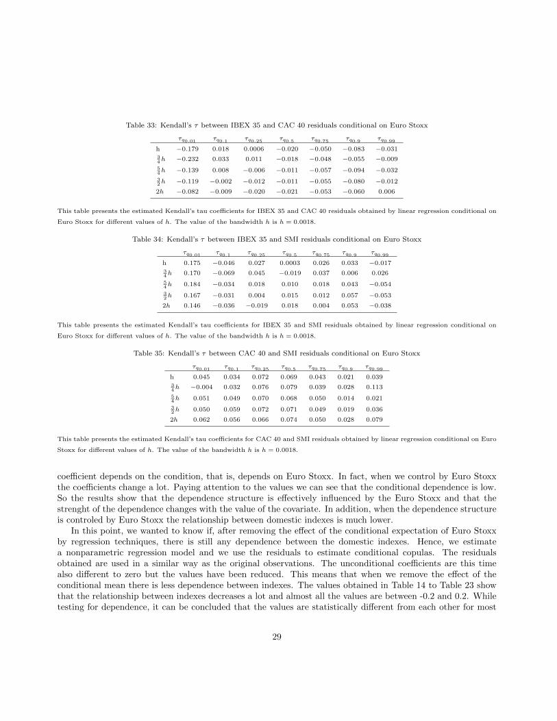
Table 33: Kendall’s τ between IBEX 35 and CAC 40 residuals conditional on Euro Stoxx

τq0.01 τq0.1 τq0.25 τq0.5 τq0.75 τq0.9 τq0.99

h −0.179 0.018 0.0006 −0.020 −0.050 −0.083 −0.03134h −0.232 0.033 0.011 −0.018 −0.048 −0.055 −0.009

54h −0.139 0.008 −0.006 −0.011 −0.057 −0.094 −0.032

32h −0.119 −0.002 −0.012 −0.011 −0.055 −0.080 −0.012

2h −0.082 −0.009 −0.020 −0.021 −0.053 −0.060 0.006

This table presents the estimated Kendall’s tau coefficients for IBEX 35 and CAC 40 residuals obtained by linear regression conditional on


Table 34: Kendall’s τ between IBEX 35 and SMI residuals conditional on Euro Stoxx

τq0.01 τq0.1 τq0.25 τq0.5 τq0.75 τq0.9 τq0.99

h 0.175 −0.046 0.027 0.0003 0.026 0.033 −0.01734h 0.170 −0.069 0.045 −0.019 0.037 0.006 0.026

54h 0.184 −0.034 0.018 0.010 0.018 0.043 −0.054

32h 0.167 −0.031 0.004 0.015 0.012 0.057 −0.053

2h 0.146 −0.036 −0.019 0.018 0.004 0.053 −0.038

This table presents the estimated Kendall’s tau coefficients for IBEX 35 and SMI residuals obtained by linear regression conditional on


Table 35: Kendall’s τ between CAC 40 and SMI residuals conditional on Euro Stoxx

τq0.01 τq0.1 τq0.25 τq0.5 τq0.75 τq0.9 τq0.99

h 0.045 0.034 0.072 0.069 0.043 0.021 0.03934h −0.004 0.032 0.076 0.079 0.039 0.028 0.113

54h 0.051 0.049 0.070 0.068 0.050 0.014 0.021

32h 0.050 0.059 0.072 0.071 0.049 0.019 0.036

2h 0.062 0.056 0.066 0.074 0.050 0.028 0.079

This table presents the estimated Kendall’s tau coefficients for CAC 40 and SMI residuals obtained by linear regression conditional on Euro

Stoxx for different values of h. The value of the bandwidth h is h = 0.0018.

coefficient depends on the condition, that is, depends on Euro Stoxx. In fact, when we control by Euro Stoxxthe coefficients change a lot. Paying attention to the values we can see that the conditional dependence is low.So the results show that the dependence structure is effectively influenced by the Euro Stoxx and that thestrenght of the dependence changes with the value of the covariate. In addition, when the dependence structureis controled by Euro Stoxx the relationship between domestic indexes is much lower.

In this point, we wanted to know if, after removing the effect of the conditional expectation of Euro Stoxxby regression techniques, there is still any dependence between the domestic indexes. Hence, we estimatea nonparametric regression model and we use the residuals to estimate conditional copulas. The residualsobtained are used in a similar way as the original observations. The unconditional coefficients are this timealso different to zero but the values have been reduced. This means that when we remove the effect of theconditional mean there is less dependence between indexes. The values obtained in Table 14 to Table 23 showthat the relationship between indexes decreases a lot and almost all the values are between -0.2 and 0.2. Whiletesting for dependence, it can be concluded that the values are statistically different from each other for most

29

of the index pairs. The results show that in those cases there is still dependence on Euro Stoxx between theindexes after removing the effect of the conditional mean. The values are not statistically signifiant only forthe relationship of SMI with FTSE 100 and IBEX 35. If we analyze the relation between SMI and FTSE 100,we can see that when Euro Stoxx takes smaller values than the mean there aren’t statistical differences in thedependence. Something similar happens with SMI and IBEX 35. In the relation between them Kendall’s tau isnot statistically significant for Euro Stoxx takes left tail values. In those two cases the dependence between theindexes is totally explained by the conditional mean for small values of Euro Stoxx. Furthermore, we wantedto see if it was necessary to remove the Euro Stoxx effect conditional mean or it was enough with removing itlinearly. When a linear regression model is used, in most of the cases the dependence between the indexes isexplained totally by the linear relationship and there is no Euro Stoxx dependence left in the residuals.

Hence, we obtain two main conclusions. First of all we conclude that the linear regression model it’s notenough and we need a more general model such as nonparametric regression models, which have the advantageof no assumptions about the functional form of the model. In addition, we also conclude that that there is stillsome dependence on Euro Stoxx between domestic indexes when we remove the effect by the conditional mean.Particularly, there is still some dependence in the left tail, that is, when Euro Stoxx takes very low values, whichis the zone that matters. Hence, it requires further research.

30

Ondorioak

Aktiboetaz hitz egiten gagozanean oso garrantzitsua da menpekotasun kontzeptua. Lan honetan indizedomestiko desberdinen arteko dagoen menpekotasuna aztertzen da indize orokorrago batera, hala nola EuroStoxx-era, baldintzatzen dogunean. Menpekotasuna aztertzeko modu bat kopulak erabiltzea da. Esan bezala,kopulak baterako banaketa funtzioak dira eta aldagai desberdinen arteko menpekotasun egitura deskribatzeaahalbidetzen dabe. Indizeen arteko menpekotasun egiturak Euro Stoxx-aren eragina jaso ahal dauanez, in-teresgarria litzateke menpekotasuna Euro Stoxx-aren balioekin zelan aldatzen dan ezagutzea. Testuinguruhonetan, baldintzatutako kopulekin lan egiten dogu. Menpekotasuna zein gogorra izan daitekeen aztertu nahidogunez, Kendall-en korrelazio koefizientea erabiltzen dogu. Euro Stoxx-arekiko menpekotasuna aztertu ahalizateko hipotesi kontraste bat diseinatu dogu, Kendall-en baldintzatu gabeko korrelazio koefizientean oinarritzendana. Gainera, konfidantza tarteetaz baliatu gara emaitzetatik ondorioak atara ahal izateko. Emaitzek esatendabenaren arabera, baldintzatutako korrelazio koefiziente guztiak desberdinak dira euren artean eta baita bald-intzatu gabeko Kendall-en koefizientearekin ere. Baldintzatu gabeko koefizientea zeroren desberdina da eta balioaltuak hartzen dauz kasu guztietan. Egia esan emaitza hau espero genduan, indizeen arteko korrelazio linealakere altuak baitira. Gainera, baldintzatutako Kendall-en koefizientea baldintzaren menpekoa da, hau da, EuroStoxx-aren menpekoa da. Izan ere, Euro Stoxx-aren balioa finkatzen dogunean koefizienteak asko aldatzen dira.Balioak arretaz begiratuz, ikus daiteke baldintzatutako menpekotasuna baxua dala. Beraz, emaitzek adieraztendaben bezala Euro Stoxx-aren balioak indizeen arteko menpekotasun egituran benetan eragina dauka eta gain-era eragin hori Euro Stoxx-ak hartutako balioen araberakoa da. Gainera, Euro Stoxx-aren balioa finkatzendogunean indizeen arteko erlazioa txikitu egiten da.

Guzti hau dala eta, indizeen artean inolako menpekotasunik dagoen jakin nahi genduan Euro Stoxx-arenbaldintzazko itxaropenaren efektua erregresio tekniken bitartez kendu ostean. Hortaz, erregresio eredu ez-parametriko bat estimatzen dogu eta hondarrak erabiltzen doguz baldintzatutako kopulak estimatzeko. Lortu-tako hondarrak jatorrizko balioak bailiran erabiltzen dira. Baldintzatu gabeko koefizienteak oraingoan ere ze-roren desberdinak dira baina balioak txikiagoak dira. Beraz, baldintzatutako batazbestekoaren efektua kentzendogunean indizeen arteko menpekotasuna gitxitu egiten da. 14. eta 23. taulen arteko balioek indizeen erlazioaasko txikitu dala erakusten dabe eta balioen gehiengoa -0.2 eta 0.2 bitartean mugitzen da. Menpekotasunarentesta egiterako orduan, ondorioztatu daiteke balioak estatistikoki desberdinak direla euren artean indize bikotegehienetarako. Emaitzek esaten dabenaren arabera, kasu honeetan oraindik indizeen artean badago Euro Stoxx-arekiko menpekotasuna baldintzatutako batazbestekoaren efektua kendu arren. SMI eta FTSE 100 arteko in-dizeen eta SMI eta IBEX 35 arteko indizeen kasuan soilik balioak ez dira estatistikoki esanguratsuak. SMI etaFTSE 100 indizeen arteko erlazioa aztertuz gero, Euro Stoxx-ak batazbestekoa baino balio txikiagoak hartzendauzanean menpekotasunean ez dago desberdintasun esanguratsurik. Antzeko zerbait gertatzen da SMI etaIBEX 35 indizeen artean. Euren arteko erlazioan Euro Stoxx-ak baliorik txikienak hartzen dauzanean Kendall-en tau koefizientea ez da esanguratsua. Bi kasu honeetan indizeen arteko menpekotasuna baldintzatutakobatazbestekoarekin guztiz azalduta dago. Gainera, Euro Stoxx-aren efektua baldintzatutako batazbestekoarekinkendu beharrean linealki kentzearekin nahikoa dan ikusi nahi izan dogu. Erregresio eredu lineal bat erabiltzendanean, gehienetan indizeen arteko menpekotasuna erlazio linealaren bitartez guztiz azaltzen da eta ez dagohondarretan Euro Stoxx-arekiko inolako menpekotasunik.

Hortaz, ondorio garrantzitsu bi lortzen doguz. Alde batetik, ez da nahikoa erregresio eredu lineal batkontsideratzearekin eta erregresio eredu ez-parametrikoa bezalako eredu orokorrago bat beharrezkoa da. Ereduez-parametrikoetan ez da forma funtzionalari buruz inolako hipotesirik egiten eta horrek abantaila bat su-posatzen dau. Beste alde batetik, indizeen artean badago oraindik nolabaiteko menpekotasuna nahiz eta bald-intzatutako batazbestekoaren efektua kendu. Bereziki, badago nolabaiteko menpekotasuna Euro Stoxx-ak baliooso txikiak hartzen dauzanean, hau da, zonalderik kritikoenean. Hortaz, ikerketa gehiago egin beharra dago.

31

References.

[1] Altman, N., Lger, C., 1994. Bandwidth Selection for Kernel Distribution Function Estimation. Journal ofStatistical Planning and Inference 46, 195-214.

[2] Blomqvist, N., 1950. On a measure of dependence between two random variables, The Annals of Mathe-matical Statistics 21, 593-600.

[3] Chan, M., Peng, L., 2002. Regression modeling for nonparametric estimation of distribution and quantilefunctions. Statistica Sinica 12, 1043-1060.

[4] Craiu, M., 2009. Parametric estimation of conditional copulas. Universitatea Politehnica din BucurestiScientific Bulletin 71, Issue 3.

[5] Croux, C., Dehon, C., 2000. Influence functions of the Spearman and Kendall correlation measures. Statis-tistical Methods and Applications 19, 497-515.

[6] Daniels, H.E., 1950. Rank correlation and population models, Journal of the Royal Statistical Society B12, 171-181.

[7] Ferreira, E., Gil, J., Orbe, S. 2011. Conditional beta pricing models: A nonparametric approach. Journalof Banking and Finance 35, 3362-3382.

[8] Fredricks, G.A., Nelsen, R.B., 2006. On the relationship between Spearman’s rho and Kendall’s tau forpairs of continuous random variables. Journal of Statistical Planning and Inference 137, 2143-2150.

[12] Gijbels, I.,Veraverbeke, N., Omelka, M., 2011a. Conditional copulas, association measures and their appli-cations. Computational Statistics and Data Analysis 55, 1919-1932.

[12] Gijbels, I.,Veraverbeke, N., Omelka, M., 2011b. Estimation of a Conditional Copula and Association Mea-sures. Scandinavian Journal of Statistics 38, 766-780.

[12] Gijbels, I.,Veraverbeke, N., Omelka, M., 2012. Multivariate and functional covariates and conditional cop-ulas. Electronic Journal of Statistics 6, 1273-1306.

[12] Gijbels, I.,Veraverbeke, N., Omelka, M., 2014. Preadjusted non-parametric estimation of a conditionaldistribution function. Journal of the Royal Statistical Society B 76, 399-438.

[13] Hansen, B.E., 2004. Bandwidth selection for nonparametric distribution estimation. University of Wiscon-sin.

[14] Herve, A., Williams, L.J., 1958. Jackknife. Encyclipedia of Research Design, SAGE publications.

[15] Hsieh, J.J., Huang, W.C., 2015. Nonparametric estimation and test of conditional Kendall’s tau undersemi-competing risks data and truncated data. Journal of Applied Statistics 42, 1602-1616.

[16] Jodgeo, K., 1982. Concepts of dependence. Encyclopedia of Statistical Sciences 1, 324-334.

[17] Krishnan, C.N.V., Petkova, R. and Ritchken, P. 2009. Correlation risk. Journal of Empirical Finance 16,353-367.

[18] Nadaraya, E.A., 1964. On estimating regression, Theory of Probability and its Applications 10, 186-190.

32

[19] Nelsen, R.B., 2012. An Introduction to Copulas, second edition. Springer, New York.

[20] Parra, H., Koodi, L., 2006. Using conditional copula to estimate Value at Risk. Journal of Data Science 4,93-115.

[21] Quenouille, M.H., 1956. Notes on bias in estimation. Biometrika 43, 353-360.

[22] Quintela, A., Estvez, G., 2012. Nonparametric Kernel Distribution Function Estimation with Kerdiest: AnR Package for Bandwidth Choice and Applications. Journal of Statistical Software 50, Issue 8.

[23] Silverman, B.W., 1986. Density estimation for statistics and data analysis. Chapman and Hall, London.

[24] Tukey, J.W., 1958. Bias and confidence in not quite large samples. Annals of Mathematical Statistics 29,614.

[25] Watson, G.S., 1964. Smooth regression analysis. Sankhya, Series A 26, 359-372.

33

Technical report

Jone Ascorbebeitia BilbatuaMaster’s Degree in Banking and Quantitative Finance

Supervisors:Eva Ferreira*

Susan Orbe-Mandaluniz 1

1UPV/EHU University of Basque Country

Kapitulua 1

Bi aldagaietako kopulak

Definizioa 1. Izan bitez S1 eta S2 R-ren azpimultzoak eta F Dom(F ) =S1×S2 eremuan definitutako funtzioa. Izan bedi baita erpin guztiakDom(F )-n daukazan J = [x1, x2]× [y1, y2] laukizuzena. Orduan, J-ren F-bolumena

VF (J) = F (x2, y2)− F (x2, y1)− F (x1, y2) + F (x1, y1)

formularen bidez emonda dago.Ohartu VF (J) J laukizuzenaren F-masa baita dala: J laukizuzenean F-renlehen ordenako deribatuak ∆x2

x1F (x, y) = F (x2, y)−F (x1, y) eta ∆y2y1F (x, y) =

F (x, y2) − F (x, y1) eran definitu badaitekez, orduan J laukizuzenaren F-bolumena J gaineko F-ren bigarren ordenako deribatua da,

VF (J) = ∆x2x1∆y2

y1F (x, y)

Definizioa 2. F aldagai biko funtzio erreala 2-gorakorra dala esaten daVF (J) ≥ 0 bada erpinak Dom(F )-n daukazan J laukizuzen guztietarako.Bestela, F n-beherakorra dala esaten da.

F 2-gorakorra danean, J laukizuzenaren F-bolumenari askotan J-ren F-neurria esaten jako. 2-gorakorrak diren funtzioei sasi monotonoak ere esatenjake. Ohartu baita F 2-gorakorra dala esateak ez dauala inplikatzen, eztainplizituki azaltzen ere ez, F argumentu bakoitzean ez-beherakorra izatea.

Adibidea 1. • Izan bedi I2 = [0, 1]2 eremuan definitutako F (x, y) =max(x, y) funtzioa. F funtzio ez beherakorra da bai x-en eta baita y-nere. Baina,VF ([0, 1]2) = ∆y2

y1∆x2x1max(x, y) = max(x2, y2)−max(x1, y2)−max(x2, y1)+

max(x1, y1) = −1 da eta hortaz, F ez da 2-gorakorra.

• Izan bedi orain I2 = [0, 1]2 eremuan definitutako F (x, y) = (2x −1)(2y − 1) funtzioa.VF ([0, 1]2) = ∆y2

y1∆x2x1 [(2x− 1)(2y− 1)] = [(2x2− 1)− (2x1− 1)][(2y2−

1) − (2y1 − 1)] = 4 ≥ 0. F funtzio 2-gorakorra da, baina x-en funtzio

i 35

ii KAPITULUA 1. BI ALDAGAIETAKO KOPULAK

beherakorra da y ∈ (0, 12) bakoitzerako eta y-n funtzio beherakorra da

x ∈ (0, 12) bakoitzerako.

Suposatu S1 eta S2-k a1 eta a2 elementu minimoak daukiezela, hurrenezhurren. F : S1 × S2 → R funtzioa oinarrituta dago (x1, x2) ∈ S1 × S2

guztietarako, F (x, a2) = 0 = F (a1, y) betetzen bada.

Lema 1.0.1. Izan bitez S1 eta S2 R-ren azpimultzo bi eta F S1 × S2 ere-muan definitutako funtzio oinarritua eta 2-gorakorra. Orduan, F argumentubakoitzean ez-beherakorra da.

Orain suposatu S1 eta S2-k b1 eta b2 elementu handien bat daukela.Orduan F : S1 × S2 → R funtzioak F1 eta F2 hurrengo marjinalak daukaz:

F1(x) = F (x, b2), x ∈ S1 guztietarako.F2(y) = F (b1, y), y ∈ S2 guztietarako.

Ohartu F1 funtzioa Dom(F1) = S1 eremuan definituta dagoela eta F2 fun-tzioa Dom(F2) = S2 eremuan.

Adibidea 2. Izan bedi [−1, 1]× [0,∞] eremuan definitutako

F (x, y) = (x+1)(ey−1)x+2ey−1 funtzioa.

F (x, 0) = 0 eta F (−1, y) = 0 betetzen diranez, F oinarrituta dago.

F-ren marjinalak hurrengoak dira:

F1(x) = F (x,∞) = (x+1)(e∞−1)x+2e∞−1 → x+1

2

F2(y) = F (1, y) = ey−1ey = 1− e−y

Definizioa 3. 2 dimentsioko azpikopula edo 2-azpikopula C ′ funtzio bat dahurrengo propietateak betetzen dauzana:

• C ′-ren eremua Dom(C ′) = S1 × S2 da, non S1 eta S2 0 eta 1 barnedaukiezan I = [0, 1]-ren azpimultzo bi diren.

• C ′ oinarritua eta 2-gorakorra da.

• u1 ∈ S1 eta u2 ∈ S2 guztietarako, C ′(u1, 1) = u1 eta C ′(1, u2) = u2.

Ohartu (u1, u2) ∈ Dom(C ′) guztietarako, 0 ≤ C ′(u1, u2) ≤ 1, beraz Ran(C ′)ere I = [0, 1]-ren azpimultzo bat da.

Definizioa 4. Bi dimentsioko kopula bat, 2-kopula bat edo beste barik ko-pula I2 = [0, 1]2 eremuan definitutako C 2-azpikopula bat da.Baliokideki, kopula bat C : [0, 1] × [0, 1] → [0, 1] eremuan definitutakoC(u1, u2) = P [U1 ≤ u1, U2 ≤ u2] funtzio bat da eta ondoko propietateakbetetzen dauz:

36

iii

1. C : [0, 1]× [0, 1]→ [0, 1].

2. C(u1, 0) = C(0, u2) = 0.

3. C(u1, 1) = u1 eta C(1, u2) = u2.

4. [0, 1] tarteko u1, u2, v1, v2 guztietarako, u1 ≤ u2 eta v1 ≤ v2 izanik:VC([u1, v1]×[u2, v2]) = C(v1, v2)−C(u1, v2)−C(v1, u2)+C(u1, u2) ≥ 0.

Nahiz eta kopula eta azpikopula kontzeptuen arteko desbardintasuna osotxikia dala iruditu, definizio eremuan dago bakarrik desbardintasuna, Sklar-en teoreman garrantzitsua izango da desbardintasun hori.

Nahiz eta kopularen kontzeptua definituta egon, badauka beste definizioformalago bat: Izan bedi C : [0, 1]× [0, 1]→ [0, 1] funtzioa.Orduan, C kopula da baldin eta soilik baldin C(u1, u2) = P (U1 ≤ u1,U2 ≤ u2), non U1, U2 ∼ U(0, 1).Beraz,

C(F1(x), F2(y)) = P (U1 ≤ F1(x), u2 ≤ F2(y)) = P (F−11 (u1) ≤ x, F−1

2 (u2) ≤ y)

= P (X ≤ x, Y ≤ y) = F (x, y)

baterako banaketa funtzioa lortzen da.

Kopulen artean ondoren aurkeztuko diran kopulak garrantzia handikoakdira. Aldagaien independentziarekin konsistentea dan kopula Π(u1, u2) =u1 · u2 biderkadura kopula da. Beraz, kasu honetan, baterako banaketafuntzioa banaketa funtzio marjinalen biderkadura izango da. Beste kopu-la garrantzitsu bat M(u1, u2) = min(u1, u2) kopula da eta Frechet-en goibornea esaten jako. Beste kopula batek ere ezin daike kopula honek bainobalio handiagoa hartu. Zorizko aldagaiak kopula honen bidez erlazionatutadagozanean menpekotasun zehatz positiboa daukela esaten da. Hirugarrenkopula garrantzitsua W (u1, u2) = max(u1 +u2−1, 0) kopula da eta Frechet-en behe bornea esaten jako. Ez dago balio txikiagoa hartu daiken bestekopularik. Zorizko aldagaiak kopula honen bidez erlazionatuta dagozaneanmenpekotasun zehatz negatiboa daukela esaten da. Esaten da kopula batekmenpekotasun positiboa edo negatiboa inplikatzen dauala Frechet-en kopu-letako batera konbergitzen badau parametroen bat aldatzen dan heinean.Gainera, (u1, u2) ∈ I2 = [0, 1]2 eta C kopula guztietarako,

W (u1, u2) ≤ C(u1, u2) ≤M(u1, u2)

Frechet-Hoeffding borneen desberdintza deitzen da.

Sklar-en teorema kopulen teoriako teorema nagusia da. Teorema honekbanaketa funtzio marjinalen eta baterako banaketa funtzioen arteko erla-zioan kopulek daukien eginkizuna argitzen dau. Sklar-en teorema aurkeztuaurretik zenbait kontzeptu gogoratuko doguz.

37

iv KAPITULUA 1. BI ALDAGAIETAKO KOPULAK

Definizioa 5. Banaketa funtzio bat R-n definitutako G funtzio bat da etapropietate bi betetzen dauz:

1. G ez-beherakorra da.

2. G(−∞) = 0 eta G(∞) = 1

Definizioa 6. Baterako banaketa funtzio bat R2-n definitutako F funtzio

bat da, non

1. F 2-gorakorra da.

2. F (x,−∞) = F (−∞, y) = 0 eta F (∞,∞) = 1

Hortaz, bigarren baldintzagatik F oinarritua da. Gainera, Dom(F ) = Rdanez, F-k F1(x) = F (x,∞) eta F2(y) = F (∞, y) moduan definitutakomarjinalak daukaz. Funtzio marjinal honeek ere banaketa funtzioak dira eraberean.

Teorema 1.0.2. (Sklar-en teorema) Izan bedi F baterako banaketa-funtziobat eta F1, F2 F-ren banaketa funtzio marjinalak. Orduan, C kopula bat exis-titzen da non x, y ∈ R guztietarako,

F (x, y) = C(F1(x), F2(y)) (1)

F1 eta F2 banaketa funtzio marjinalak jarraituak badira orduan C kopulabakarra da eta hortaz modu unibokoan zehaztuta dago ran(F1) × ran(F2)eremuan. Alderantziz, C kopula bat bada eta F1 eta F2 banaketa funtzioakbadira, orduan (1) adierazpenean definitutako F funtzioa banaketa funtziobateratua da F1 eta F2 marjinalekin.

Sklar-en teoremak baterako banaketa funtziorako adierazpen bat emotendau kopularen eta banaketa funtzio marginal biren menpean. Adierazpenhorri buelta emonez gero, kopula baterako banaketa funtzioaren eta funtziomarjinalen alderantzizkoen menpe jarri daitekez. Hala ere, banaketa fun-tzio marjinalen bat hertsiki gorakorra ez bada, orduan alderantzizkoak ezdauka ohiko zentzua. Hori dala eta, banaketa funtzioen ”sasi alderantziz-koak”definitzea beharrezkoa da.

Definizioa 7. Izan bedi F banaketa funtzioa. Orduan, F-ren sasi alderan-tzizkoa hurrengo bi propietateak betetzen dauzan [0, 1] tartean definitutakoedozein F (−1) funtzio da:

• t ∈ Im(F ) eta x ∈ R badira, F (−1)(t) = x y F (x) = t. Hortaz,t ∈ Im(F ) guztietarako,

F (F (−1)(t)) = t

38

v

• t 6∈ Im(F ) bada, F (−1)(t) = inf{x : F (x) ≥ t} = sup{x : F (x) ≤ t}.

F hertsiki gorakorra danean sasi alderantzizkoa ohiko alderantzizko funtzioada.

Sklar-en alderantzizko teoremaren arabera, edozein motatako banaketafuntzio bi bateratu daitekez (ez da beharrezkoa familia bardinekoak izatea)edozein kopularekin; eta ondorioz aldagai biko banaketa funtzio baliagarribat definituta egongo da. Zein da emaitza honen erabilgarritasuna? Ekono-mia eta estatistikan aldagai bakarreko banaketa funtzio parametriko ugaridagoz, baina aldagai anitzeko banaketa funtzioen multzoa oso txikia da.Izan ere, baliteke aldagai anitzeko banaketa funtzioen konplexutasunak edofuntzio honeen iraganeko erabilera eskasak arazo hau sortarazo izana. Halaere, Hutchinson eta Lai (1990), Joe Clyton (1997) eta Nelsen-en (1999) la-netan ikusi daitekeen moduan, kopula parametriko ugari dagoz aldagai ani-tzeko dentsitate funtzioen modelizaziorako. Orduan, aipatutako funtzioakbakarrik erabilita aldagai anitzeko banaketa funtzio parametriko posibleenmultzoa izugarri handitzen da Sklar-en teoremari esker. Ideia bat egin ahalizateko izan bitez M, N eta P aldagai anitzeko banaketa funtzio, aldagai ba-karreko banaketa funtzio eta kopula kopurua hurrenez hurren. Esandakoa-ren arabera, N >> M da. Sklar-en teoremarekin aldagai anitzeko banaketafuntzio parametrikoen kopurua M izatetik N2 · P >> M izatera pasatu da.Argi dago banaketa funtzio guzti honeek ez dirala enpirikoki erabilgarriak,baina aukera multzoa handitzeak datuekiko egokitze aproposa emoten da-ben ereduak aurkitzeko aukera hobetzen dau.

Korolarioa 1.0.3. Izan bitez H bi aldagaiko banaketa funtzioa eta F eta Gbere banaketa funtzio marjinal jarraituak. Izan bitez baita F (−1) eta G(−1)

banaketa funtzio marjinalen sasialderantzizkoak. Orduan, C : [0, 1]×[0, 1]→[0, 1] kopula bakarra existitzen da non

C(u1, u2) = H(F (−1)(u1), G(−1)(u2)), (u1, u2) ∈ [0, 1]× [0, 1]guztietarako.

Sklar-en teoremaren korolario honek hurrengoa dino: aldagai anitzekoedozein banaketa funtzioren kopula ataratzea posiblea da eta funtzio haujatorrizko banaketa funtzioaren marjinalak edozein direlarik erabilten da.Hortaz, propietate honetan ikusi daiteke aldagai anitzeko banaketa funtzioenmultzoa are gehiago handitzen dala.

Orduan, Sklar-en alderantzizko teorematik edozein banaketa funtzio mar-jinal bi eta kopula bat emonda banaketa funtzio bateratua lortu daiteke.Aurreko korolarioari esker, edozein baterako banaketa funtziorako kopulainplizitua eta banaketa funtzio marjinalak lortu daitez.

Oharra 1. Izan bitez X eta Y zorizko aldagaiak eta suposatu hurrengoadierazpena:

39

vi KAPITULUA 1. BI ALDAGAIETAKO KOPULAK

F (x, y) = C(FX(x), FY (y))

Sklar-en teorema jarraituz, baterako probabilitatea kopula eta marjinalenartean banantzen da eta kopulak X eta Y-ren arteko lotura bakarrik adie-razten dau. Banaketa funtzioaren bitartez adierazitako probabilitate ba-teratuan ez bezala, kopulek portaera marjinala multzotik banantzen dabe.Hori dala eta, kopulak menpekotasun funtzio bezala izendatzen dira. Kasuhonetan, C kopulari X eta Y zorizko aldagaien arteko kopula esaten jako etaCXY adierazten da.

Proposizioa 1.0.4. • Izan bedi CXY X eta Y-ren kopula eta α eta βfuntzio hertsiki gorakorrak. Orduan, Cα(X)β(Y ) = CXY . Hortaz, CXYinbariantea da X eta Y-ren edozein transformazio hertsiki gorakorre-rako.

• Izan bitez C1 eta C2 bi kopula. Orduan, C1 C2 baino txikiagoa da (etaC1 ≺ C2 idazten da) C1(u1, u2) ≤ C2(u1, u2) bada u1, u2 ∈ I = [0, 1]guztietarako.

Kopula baten dentsitatea definitu ahal izateko, lehenik eta behin teoremabat beharrezkoa da.

Teorema 1.0.5. Izan bedi C kopula bat. u1, u2 ∈ I = [0, 1] guztietarako ∂C∂u1

deribatu partziala existitzen da eta u1 eta u2 horreetarako

0 ≤ ∂C(u1,u2)∂u1

≤ 1.

Era berean, u1, u2 ∈ I = [0, 1] guztietarako ∂C∂u1

deribatu partziala existitzenda eta u1 eta u2 horreetarako

0 ≤ ∂C(u1,u2)∂u2

≤ 1.

Gainera, u1 7→ ∂C(u1,u2)∂u2

eta u2 7→ ∂C(u1,u2)∂u1

funtzioak ez beherakorrak diraeta definituta dagoz I = [0, 1] eremuan.

Definizioa 8. Kopula baten dentsitatea, c adierazten dana, hurrengo adie-razpenarekin definitzen da:

c(u1, u2) =∂C(u1, u2)

∂u1∂u2(2)

c(u1, u2) kopularen dentsitatea eukinda F banaketa funtzioaren f dentsitatefuntzioa hurrengo eran lortu daiteke:

f(x, y) = c(FX(x), FY (y)) · fX(x) · fY (y) (3)

Azken adierazpen hau Sklar-en kopulen dentsitateetarako teorema moduanere ezagutzen da.

40

1.1. KOPULA ELIPTIKOAK vii

1.0.1 Kopula motak

Kopula funtzio mota desbardin asko dagoz baina zaila da mota guztie sail-kapen zehatz bat aurkitzea, irizpide desbardinak baitagoz. Kopulak menpe-kotasunaren arabera, euskarriaren arabera (jarraitua edo diskretua), etab.sailkatu daitekez.

• Kopula inplizitua edo esplizitua

– Kopula inplizituak: Kopularen forma funtzionalak bat egiten daubanaketa funtzio ezagun bategaz (Gauss-en kopula, student-en tkopula).

– Kopula esplizituak: Kopula bakoitzak forma funtzional erraz batdauka (Gumbel, Clayton eta Frank-en kopulak) .

• Menpekotasunaren arabera sailkatutako kopulak: Kopula eliptikoak,kopula normalak, mutur balioetako kopulak, kopula arkimedearrak etaHRT kopulak.

Orain kopula desbardinak aztertuko dira.

1.1 Kopula eliptikoak

Definizioa 9. Kopula eliptikoak banaketa funtzio eliptikoekin lotutako ko-pulak dira. Kopula eliptikoek menpekotasun erlazio simetrikoak adieraztendabez, banaketa funtzioaren ezkerreko zein eskumako aldea aztertzen danarduratu barik. Kopula eliptiko guztiek itxura bera daukie:

Cρ(u1, u2) =1√

1− ρ2

∫ Φ−1g,1(u1)

−∞

∫ Φ−1g,2(u2)

−∞g(x2 − ρxy + y2

√1− ρ2

)dx · dy

= Hρ(Φ−1g,1(u1),Φ−1

g,2(u2))

Gauss-en eta Student-en t kopulak kopula eliptikoak dira, simetrikoaketa erabiltzerako orduan errazak dira lotuta dagozan banaketak ezagunakdirelako.

Aipatu bezala, kopula normala edo Gauss-en kopula eta Student-en tkopula kopula elptiko ezagunenak dira.

1.1.1 Gauss-en kopula

Gauss-en kopula banaketa funtzio normalari lotutako menpekotasun fun-tzioa da eta kopula mota hau kopula inplizitua da. Izan bedi ρ positiboki

41

viii KAPITULUA 1. BI ALDAGAIETAKO KOPULAK

definitutako matrize diagonala non diagonaleko elementuak 1 diren. Or-duan, Gauss-en kopula hurrengo eran definitzen da:

C(u1, u2; ρ) = Φρ(Φ−1(u1),Φ−1(u2))

=

∫ Φ−1(u1)

0

∫ Φ−1(u2)

0

1

2π√

1− ρ2exp(−x

21 + x2

2 − 2ρx1x2

2(1− ρ2)dx1dx2

(4)

Gainera, kopula mota honen dentsitatea

c(u1, u2; ρ) =1√

1− ρ2exp(

x21 + x2

2 − 2ρx1x2

2(1− ρ2)+x2

1 + x22

2)

Gauss-en kopula kopula simetrikoa da, hau da, C(u1, u2) = C(u2, u1). Ko-pula honek alboetan menpekotasun nulua edo oso baxua dauka, aldagaienkorrelazioa 1 ez bada. Beraz, finantza-errentagarritasunen menpekotasu-na modelizatzeko ez da kopula oso egokia. Gainera, badirudi finantza-errentagarritasunak handiagoak eta negatiboak direnean korrelazio handia-goa daukela handiak eta positiboak direnean baino, alboetako menpekota-suna asimetrikoa dala aditzera emoten dauana.

1.1.2 Student-en t kopula

Student-en t kopula Student-en t banaketa funtzioari lotutako menpeko-tasun funtzioa da eta hau ere kopula inplizitua da. Aldagai biren kasuanondoko eran definitzen da:

C(u1, u2; ρ, ν) = tρ,ν(t−1(u1), t−1(u2)) (5)

Lehenik eta behin Student-en t banaketaren dentsitatea ezagutzea beha-rrezkoa da kopula definitu ahal izateko. Gogoratu kopulak aldagaitzak direlatransformazio gorakor monotonoetarako, C(t(ν, µ,Σ)) = C(t(ν, 0, P )) eta Pkorrelazio matrizea. Beraz,

f(x) = 1

2π√

1−ρ2(1 +

x21−2ρx1x2+x22ν(1−ρ2)

)−ν+22 da,

non ν askatasun graduak eta ρ korrelazio koefizientea diren. Student-en t

banaketak orokorrean Xd= µ+

√νS ·Z adierazpena dauka, non Z ∼ N(0,Σ)

dan. Beraz, Studen-en t kopula ondoko eran definitu daiteke:

C(u1, u2) = tν(t−1ν1 (u1), t−1

ν2 (u2)) =

∫ t−1ν (u1)

−∞

∫ t−1ν (u2)

−∞f(x)dx

=

∫ t−1ν (u1)

−∞

∫ t−1ν (u2)

−∞

1

2π√

1− ρ2(1 +

x21 − 2ρx1x2 + x2

2

ν(1− ρ2))−

ν+22 dx

(6)

42

1.2. MUTUR BALIOETAKO KOPULAK ix

eta Student-en t kopularen dentsitatea

c(u1, u2) = K1√

(1− ρ2)[1+

x21 − 2ρx1x2 + x2

2

ν(1− ρ2)]−

ν+22 [(1+ν−1x2

1)(1+ν−1x22)]

ν+12

(7)formularen bidez emonda dago, non K = ν

2 Γ(ν2 )2Γ(ν+12 )−2 eta ν kopularen

askatasun gradu kopurua diren.

1.2 Mutur balioetako kopulak

Mota honetako kopulak oso erabilgarriak dira banaketa funtzio marginale-tan muturretako gertaerei garrantzi handiagoa emoten erlazioak adierazte-ko. Mutur balioetako kopulak askeak eta berdinki banatutako laginen maxi-moei lotutako kopulen limiteak dira, beti ere limitea existitzen dan kasuetan.Izan bedi bi dimentsiotako zorizko aldagaiez sortutako (X1, Y1), ..., (Xn, Yn)lagina, non aldagaiak askeak eta berdinki banatuak diren FX eta GY mar-ginalekiko eta HXY baterako banaketarekiko. Sklar-en teoremaren arabe-ra HXY baterako banaketa funtzioari C kopula bat lotzen jako: HXY =C(FX(x), GY (y)). Izan bitezMn = max{X1, ..., Xn} etaNn = max{Y1, ..., Yn}bi aldagai, Fn(x) = P [Mn ≤ x] eta Gn(y) = P [Nn ≤ y] euren banaketa fun-tzioak hurrenez hurren eta Hn(x, y) = P [Mn ≤ x,Nn ≤ y] baterako bana-keta funtzioa. C (Mn, Nn) bikoteari eta bere limiteari lotutako kopula bada(n-k infinitorantz joten dauanean), orduan C mutur balioko kopula bat da-la esaten da. Mutur balioko kopulek menpekotasun positiboa modelizatzendabe.

Dehuelves- en teoremaren arabera mutur balioko C kopula batek hurren-go baldintza bete behar dau:

Ct(u1t1 , u

1t2 ) = C(u, v), para todo t > 0

Mota honetako kopulek , Pickands-en (1981) hurrengo teoreman azaltzendan bezala, adierazpen bat daukie lotuta.

Teorema 1.2.1. Mutur balioko kopulen adierazpena C kopula bat mu-tur balioko kopula bat da baldin eta soilik baldin hurrengo erlazioa betetzendauan [0, 1] tartean definitutako A funtzio erreal bat existitzen bada:

C(u1, u2) = exp{−log(u1 · u2) ·A(log(u2)

log(u1 · u2))} (8)

edo baliokideki:

C(e−u1 , e−u2) = exp{−(u1 + u2) ·A(u2

log(u1 + u2))} (9)

A funtzioa Pickands-en menpekotasun funtzioa da eta hurrengo baldin-tzak betetzen dauz:

43

x KAPITULUA 1. BI ALDAGAIETAKO KOPULAK

• Ganbila da [0, 1] tartean.

• max(t, 1− t) ≤ A(t) ≤ 1, t ∈ [0, 1] guztietarako.

1.3 Kopula arkimedearrak

Kopula arkimedearrak, finantzetako eta geoestatistikako arloetan erabiliakizan aurretik, beste arlo batzuetan aplikatuak izan ziran Clayton, Oakes etaCook eta Johnsonengatik. Arrazoi asko dira kopula arkimedearrak hain-beste erabili izana. Inplementatzeko, bornatzeko eta simulazio desberdinakegiteko erraztasuna eta baita malgutasuna edo daukiezan propietate ma-tematikoak egiten dabez erakargarriak mota honetako kopulak. Hala ere,kopula arkimedearrek badaukie desabantailaren bat. Hain zuzen, argumen-tuekiko simetria, hau da, C(u1, u2) = C(u2, u1).

Definizioa 10. Izan bedi Ψ ψ : [0, 1] → [0,∞) funtzioen multzoa. ψ fun-tzioak jarraituak, hertsiki beherakorrak eta ganbilak dira eta ψ(0) =∞ etaψ(1) = 0. Orduan Ψ multzoko ψ funtzio bakoitzak hurrengo adierazpenajarraitzen dauan C kopula bat sorrarazten dau:

C(u1, u2) = ψ−1(ψ(u1) + ψ(u2)), non 0 ≤ u1, u2 ≤ 1

ψ funtzioari kopularen sortzailea esaten jako eta ψ−1 ψ funtzioaren sa-sialderantzizkoa hurrengo eran dago definituta:

ψ−1(t) =

ψ−1(t) 0 ≤ t < ψ(0)

0 ψ(0) ≤ t <∞

Aurrerago ikusiko dan moduan, kopula arkidemedearren adierazpenakaldagai anitzeko kopula baten ikerketa aldagai bakarreko funtzio batera mu-rrizten dau. Esan bezala, ψ funtzioa C kopularen sortzaile arkimedearra da.ψ(0) =∞ bada, C kopula hertsiki arkimedearra dala esaten da.

Orain ikusi daiguzan kopula arkimedearren familian parte hartzen dabenkopula mota batzuk.

1.3.1 Kopula independentea

Kopula independentearen kasuan funtzio sortzailea ψ(t) = −ln t da etahortaz, bere alderantzizkoa ψ−1(x) = e−x. Orduan, eta aurrekoa kontuanhartuz, kopula independentearen adierazpena lortu daiteke:

C(u1, u2) = ψ−1(ψ(u1) + ψ(u2)) = ψ−1(−ln u1 − ln u2)

= ψ−1(−(ln u1 + ln u2)) = ψ−1(−ln (u1u2)) = e−(−ln u1u2)

= u1 · u2

(10)

44

1.3. KOPULA ARKIMEDEARRAK xi

Aurreko adierazpena u1-ekiko deribatzen da C1 lortzeko:

C1(u1, u2) = (∂C(u1, u2)

∂u1) = u2 (11)

Orduan kopularen dentsitatea:

c(u1, u2) = (∂C(u1, u2)

∂u1∂u2) = 1 (12)

Kontuan hartu, kopula independentea aurrerago definitutako Π(u1, u2) =u1 · u2 biderkadura kopula dala.

1.3.2 Frank kopula

Frank kopularen kasuan funtzio sortzailea hurrengoa da:

ψ(t) = −lne−δt − 1

e−δ − 1, δ ∈ R (13)

Orduan, ψ−1 alderantzizko funtzioa ψ−1(x) = −1δ ln[1 + e−δ−1

ex ] dala on-dorioztatu daiteke.

Hortaz, Frank kopula hurrengo eran definitzen da:

C(u1, u2) = ψ−1(ψ(u1) + ψ(u2)) = ψ−1(−lne−δu1 − 1

e−δ − 1− lne

−δu2 − 1

e−δ − 1)

= ψ−1(ln(e−δ − 1)2

(e−δu1 − 1)(e−δu2 − 1))

= −1

δln(1 +

(e−δu1 − 1)(e−δu2 − 1)

e−δ − 1)

(14)

C(u1, u2) kopula funtzioa u1-ekiko deribatuz gero:

C1(u1, u2) = (∂C(u1, u2)

∂u1) = e−δu1

e−δu2 − 1

(e−δ − 1) + (e−δu1 − 1)(e−δu2 − 1)(15)

Orduan dentsitate funtzioa hurrengoa izango litzateke:

c(u1, u2) = (∂C(u1, u2)

∂u1∂u2) =

−δe−δu1e−δu2(e−δ − 1)

[(e−δ − 1) + (e−δu1 − 1)(e−δu2 − 1)]2(16)

45

xii KAPITULUA 1. BI ALDAGAIETAKO KOPULAK

1.3.3 Gumbel kopula

Gumbel kopula kopula arkimedear mota bat da. Kasu honetan funtzio sor-tzailea ψ(t) = (−ln t)δ da, non δ ≥ 1 dan. ψ funtzioaren alderantzizkoa

ψ−1(x) = exp(−x 1δ ). Orduan,

C(u1, u2) = ψ−1(ψ(u1) + ψ(u2)) = ψ−1((−ln u1)δ + (−ln u2)δ)

= exp(−[(−ln u1)δ + (−ln u2)δ]1δ )

(17)

Aurreko adierazpen hau u1-ekiko deribatuz gero:

C1 = (∂C(u1, u2)

∂u1) = C(u1, u2)[(−ln u1)δ + (−ln u2)δ]−1+ 1

δ−ln uδ−1

1

u1(18)

Beraz, kopularen dentsitatea hurrengoa da:

c(u1, u2) = (∂C(u1, u2)

∂u1∂u2)

= C(u1, u2)[(−ln u1)δ + (−ln u2)δ]2δ

+2[ln u1 · ln u2]δ−1·· {1 + (δ − 1)[(−ln u1)δ + (−ln u2)δ]−

1δ }

Gumbel kopulak menpekotasun positiboa dauka goiko buztanean δ > 1bada. δ-k balio desberdinak hartzen dauzan heinean Gumbel kopula inde-pendentzia (δ = 1) eta menpekotasun zehatz positiboaren artean mugitzenda, δ → ∞ danean Gumbel kopulak Frecheten goi borneko kopulara kon-bergitzen baitau.

1.3.4 Clayton kopula

Clayton kopularen kasuan funtzio sortzailea ψ(t) = 1δ (t−δ − 1) da. ψ fun-

tzioaren alderantzizkoa ψ−1(x) = (δx+ 1)−1δ . Orduan,

C(u1, u2) = ψ−1(ψ(u1) + ψ(u2)) = ψ−1(1

δ(u−δ1 − 1) +

1

δ(u−δ2 − 1))

= ψ−1(1

δ(u−δ1 + u−δ2 − 2)) = (u−δ1 + u−δ2 − 1)−

1δ

(19)

Adierazpen hau u1-ekiko deribatzen bada:

C1 = (∂C(u1, u2)

∂u1) = u−δ−1

1 (u−δ1 + u−δ2 − 1)−1− 1δ (20)

Hortaz, Clayton kopularen dentsitatea:

46

1.4. KOPULA BALDINTZATUAK xiii

c(u1, u2) = (∂C(u1, u2)

∂u1∂u2) = (u1u2)−δ−1(δ + 1)(u−δ1 + u−δ2 − 1)−2− 1

δ (21)

Clayton kopulak menpekotasun asimetrikoa dauka buztanetan. Kopulamota honek menpekotasun nulua dauka goiko buztanean eta menpekotasunpositiboa beheko buztanean δ > 0 danean. δ-ren balio desberdinetarakoClayton kopulak menpekotasun gradu desberdinak hartu daikez. Menpeko-tasuna zehatz positiboa izango da δ → ∞ doan heinean, Gumbel kopulanbezala Frecheten goi borneko kopulara konbergitzen baitau.

1.4 Kopula baldintzatuak

Orain, zorizko aldagaien erlazioa aztertzeaz gain, koaldagai baten balioaemonda erlazio hori koaldagaiaren balio desberdinekin zelan aldatzen danaztertzea izango da helburua. Izan bitez X,Y zorizko aldagaiak eta Z = zkoaldagaia. Aurrerago ikusiko dan moduan, Z = z emonda, X eta Y -ren menpekotasun egitura kopula baldintzatua izeneko funtzio baten bidezdeskribatzen da. Orduan, (X,Y ) aldagaien baterako banaketa funtzioa etafuntzio marjinalak, Z = z baldintzapean,

Fz(x, y) = P (X ≤ x, Y ≤ y|Z = z),F1z(x) = P (X ≤ x|Z = z) eta F2z(y) = P (Y ≤ y|Z = z).

dira hurrenez hurren.

Definizioa 11. U1 eta U2-rekiko deribatu partzialek C kopulari loturikokopula baldintzatuak definitzen dabez (C kopularen monotonia dala eta, u1

eta u2 ia guztietarako existitzen dira):

• u1 finko baterako, u1-rekiko kopula baldintzatua U2-ren funtzio batda, u2 → C1(u1, u2) = C(u2|u1) = ∂C

∂u1(u1, u2)

• u2 finko baterako, u2-rekiko kopula baldintzatua U1-ren funtzio batda, u1 → C2(u1, u2) = C(u1|u2) = ∂C

∂u2(u1, u2)

Definizioa 12. Aldagai biko banaketa funtzio baldintzatua eskuinetik ja-

rraitua dan Fz : R2 → [0, 1] funtzioa da eta ondoko propietateak betetzen

dauz:

• Fz(y1,−∞|Z = z) = Fz(−∞, y2|Z = z) = 0 eta Fz(∞,∞|Z = z) = 1

• x1, x2, y1, y2 ∈ R guztietarako eta x1 ≤ x2, y1 ≤ y2,VFz([x1, x2]×[y1, y2]) ≡ Fz(x2, y2|Z = z)−Fz(x1, y2|Z = z)−Fz(x2, y1|Z =z) + Fz(x1, y1|Z = z) ≥ 0.

47

xiv KAPITULUA 1. BI ALDAGAIETAKO KOPULAK

Lehenengo baldintzak banaketa funtzioaren goi eta behe borneak emotendauz. Bigarren baldintzan aldiz, [x1, x2]× [y1, y2] eremuko edozein punturenprobabilitatea ez-negatiboa dala ziurtatzen da.

Definizioa 13. Kopula baldintzatu bat Cz : [0, 1] × [0, 1] → [0, 1] funtziobat da hurrengo propietateak betetzen dauzana:

1. Cz(u1, 0|Z = z) = Cz(0, u2|Z = z) = 0, u1, u2 ∈ [0, 1] guztietarako.

2. Cz(u1, 1|Z = z) = u1 eta Cz(1, u2|Z = z) = u2, u1, u2 ∈ [0, 1] guztie-tarako.

3. [0, 1] tarteko u1, u2, v1, v2 guztietarako, u1 ≤ u2 eta v1 ≤ v2 izanik:VCz([u1, v1]× [u2, v2]|Z = z) ≡ Cz(v1, v2|Z = z)− Cz(u1, v2|Z = z)−Cz(v1, u2|Z = z) + Cz(u1, u2|Z = z) ≥ 0.

Oraingoan ere lehenengo baldintzak banaketa funtzioaren goi eta beheborneak emoten dauz. Gainera, Cz(u1, 1|Z = z) eta Cz(1, u2|Z = z) ba-naketa marjinalak uniformeak izatea ziurtatzen dau. Bigarren baldintzak,lehengo legez, puntu baten probabilitatearen ez negatibotasuna adieraztendau.

Aurreko baldintza biak R2

eremura hedatuz, kopula baldintzatua (U1t, U2t)zorizko aldagaien baterako banaketa funtzio baldintzatua moduan definitudaiteke, non marjinalak Unif(0, 1) banaketa uniformea jarraitzen daben:

C∗z (u1, u2|Z = z) =

0 u1 < 0 edo u2 < 0,

Cz(u1, u2|Z = z) (u1, u2) ∈ [0, 1]× [0, 1],

u1 u1 ∈ [0, 1], u2 > 1,

u2 u1 > 1, u2 ∈ [0, 1],

1 u1 > 1, u2 > 1,

2-kopula baterako kopula baldintzatu biren banaketa funtzioak definitudaitekez:

C(u1|u2) = P (U1 < u1|U2 = u2)

C(u2|u1) = P (U2 < u2|U1 = u1)

Arinago ikusitako Sklar-en bi teoremetatik aparte, badago kopula bal-dintzatueri egokitutako Sklar-en teorema bat ere.

48

1.4. KOPULA BALDINTZATUAK xv

Teorema 1.4.1. Izan bitez Fz aldagai biren baterako banaketa funtzioa etaF1z eta F2z bere marjinal jarraituak. Orduan, Cz : [0, 1]× [0, 1]→ [0, 1] ko-pula baldintzatu bakarra existitzen da non x, y ∈ R = [−∞,∞] guztietarako,

Fz(x, y|Z = z) = Cz(F1z(x|Z = z), F2z(y|Z = z)|Z = z) (22)

Alderantziz, Cz kopula baldintzatua eta F1z eta F2z X eta Y zorizko al-dagai biren marjinal baldintzatuak badira, orduan (22) ekuazioarekin defini-tutako Fz funtzioa F1z eta F2z marjinalak daukazan banaketa funtzio baldin-tzatua da.

49

xvi KAPITULUA 1. BI ALDAGAIETAKO KOPULAK

50

Kapitulua 2

Aldagai anitzeko kopulak

Atal honetan aurreko ataletako emaitzak aldai anitzeko kasura luzatuko do-guz. Egia esan, definizio eta teorema asko antzekoak dira aldagai anitzekobertsioan. Hala ere, ez da kasu guztietan emoten eta hori dala eta kontuhandiz jokatu behar da.Lehenik eta behin, aurrerago baliagarriak izango diran zenbait kontzeptudefinituko dira.

Definizioa 14. Izan bedi n zenbaki oso positibo bat. n-kutxa bat R-ko ntarte itxiren arteko edozein biderketa kartesiarra da. J = [a1, b1] × ... ×[an, bn] edozein n-kutxa J = [(a1, ..., an), (b1, ..., bn)] ere idazten da. ai = aeta bi = b bada i = 1, ..., n guztietarako, J = [a, b]n idatzi daiteke.

Gainera, esaten da J n-kutxa endekatua dala existitzen bada i, 1 ≤ i ≤n, non ai = bi. Bestela, J n-kutxa ez endekatua edo endekatu gabea dalaesaten da. Beste alde batetik, J-ren erpinak (c1, ..., cn) puntuak dira, noni = 1, ..., n bakoitzerako ci = ai edo ci = bi. J endekatu gabea bada, orduan2n erpin daukaz.

Definizioa 15. Izan bitez S1, S2, ..., Sn R-ren azpimultzoak eta F n-dimentsi-oko funtzio errala non Dom(F ) = S1×S2× ...×Sn. Izan bedi baita erpinakDom(F )-n dauzan J n-kutxa endekatu gabea. Orduan, J n-kutxaren F-bolumena hurrengo eran emonda dago:

VF (J) =∑

sgn(c)F (c), (1)

non batukaria J-ren c erpin guztien gainean hartzen dan eta sgn(c)

sgn(c) =

1 ck = ak bada k indize kopurua bikoitia danean

−1 ck = ak bada k indize kopurua bakoitia danean

moduan definituta dagoen.

xvii 51

xviii KAPITULUA 2. ALDAGAI ANITZEKO KOPULAK

J=[a,b]-ren F-bolumena beste modu baliokide baten ere definitu daiteke.Hain zuzen, J-ren F-bolumena F-ren J gaineko n ordenako aldakuntza da,hau da,

VF (J) = ∆baF (t) = ∆bn

an∆bn−1an−1

...∆b2a2∆b1

a1F (t), (2)

non lehenengo ordenako n aldakuntzak

∆bkakF (t) = F (t1, ..., tk−1, bk, tk+1, ..., tn)− F (t1, ..., tk−1, ak, tk+1, ..., tn) (3)

moduan definituta dagozan.

Adibidea 3. Izan bitez F R3-ko funtzioa eta J [x1, x2] × [y1, y2] × [z1, z2]

3-kutxa. Orduan, J-ren F-bolumena:

VF (J) = ∆baF (t) = ∆b3

a3∆b2a2∆b1

a1F (t)

= ∆b3a3∆b2

a2 [F (b1, t2, t3)− F (a1, t2, t3)]

= ∆b3a3{[F (b1, b2, t3)− F (b1, a2, t3)]− [F (a1, b2, t3)− F (a1, a2, t3)]}

= ∆b3a3{F (b1, b2, t3)− F (b1, a2, t3)− F (a1, b2, t3) + F (a1, a2, t3)}

= [F (b1, b2, b3)− F (b1, b2, a3)]− [F (b1, a2, b3)− F (b1, a2, a3)]

− [F (a1, b2, b3)− F (a1, b2, a3)] + [F (a1, a2, b3)− F (a1, a2, a3)]

= F (b1, b2, b3)− F (b1, b2, a3)− F (b1, a2, b3) + F (b1, a2, a3)

− F (a1, b2, b3) + F (a1, b2, a3) + F (a1, a2, b3)− F (a1, a2, a3)

Kontuan izanda kasu honetan a = (a1, a2, a3) = (x1, y1, z1) eta b = (b1, b2, b3)= (x2, y2, z2) direla:

VF (J) = F (x2, y2, z2)− F (x2, y2, z1)− F (x2, y1, z2) + F (x2, y1, z1)

− F (x1, y2, z2) + F (x1, y2, z1) + F (x1, y1, z2)− F (x1, y1, z1).

Definizioa 16. F n aldagaiko funtzio erreala n-gorakorra dala esaten daVF (J) ≥ 0 bada erpinak Dom(F )-n daukazan J n-kutxa guztietarako. Bes-tela, F n-beherakorra dala esaten da.

F funtzioa n-beherakorra da baldin eta soilik baldin -F n-gorakorra bada.Beste alde batetik, J kutxa endekatu gabea bada, orduan VF (J) = 0 da.Suposatu F n aldagaiko funtzio erreal baten eremua Dom(F ) = S1× ...×Sndala non Sk bakoitzak ak elementu minimo bat daukan.F oinarrituta dagoelaesaten da gitxienez k baterako tk = ak diren t ∈ Dom(F ) guztietarakoF (t) = 0 bada. Sk bakoitza ez-hutsa bada eta bk elementu handien batbadauka, orduan F-k marjinalak daukaz. F-ren dimentsio bateko marjinalakDom(Fk) = Sk eremuan definitutako Fk funtzioak dira,

Fk(x) = F (b1, ..., bk−1, x, bk+1, ..., bn), x ∈ Sk guztietarako. (4)

Adibidea 4. Izan bedi [−1, 1]× [0,∞]× [0, π2 ] eremuan definitutako

52

xix

F (x, y, z) = (x+1)(ey−1)sin zx+2ey−1 funtzioa.

F (x, y, 0) = 0, F (x, 0, z) = 0 eta F (x, y, 0) = 0 betetzen diranez, F oina-rrituta dago.

F-ren dimentsio bateko marjinalak hurrengoak dira:

F1(x) = F (x,∞, π2 ) = (x+1)(e∞−1)x+2e∞−1 → x+1

2

F2(y) = F (1, y, π2 ) = ey−1ey = 1− e−y

F3(z) = F (1,∞, z) = e∞−1e∞ sin z = sin z

F-ren bi dimentsiotako marjinalak:

F1,2(x, y) = F (x, y, π2 ) = (x+1)(ey−1)x+2ey−1

F2,3(y, z) = F (1, y, z) = ey−1ey sin z = (1− e−y)sin z

F1,3(x, z) = F (x,∞, z) = (x+1)(e∞−1)sin zx+2e∞−1 → (x+1)sin z

2

Aurrerantzean dimentsio bateko marjinalei marjinala bakarrik esangojake eta k ≥ 2 danean k dimentsioko marjinalak k-marjinalak izango dira.

Lema 2.0.2. Izan bitez S1, ..., Sn R-ren azpimultzo es hutsak eta F funtzion-gorakor oinarritua S1× ...×Sn eremuarekin. Orduan, F ez-beherakorra daargumentu bakoitzean; hau da, (t1, ..., tk−1, x, tk+1, ..., tn) eta (t1, ..., tk−1, y,tk+1, ..., tn) F-ren eremuan badagoz eta x < y bada, orduan

F (t1, ..., tk−1, x, tk+1, ..., tn) ≤ F (t1, ..., tk−1, y, tk+1, ..., tn).

Definizioa 17. n dimentsioko azpikopula edo n-azpikopula C ′ funtzio batda hurrengo propietateak betetzen dauzana:

• C ′-ren eremua Dom(C ′) = S1 × ... × Sn da, non Sk bakoitza 0 eta 1barne daukazan I = [0, 1]-ren azpimultzo bat dan.

• C ′ oinarritua eta n-gorakorra da.

• C ′-k (dimentsio bateko) C ′k marjinalak daukaz, k = 1, ..., n eta u ∈ Skguztietarako C ′k(u) = u betetzen dabe.

Ohartu u ∈ Dom(C ′) guztietarako 0 ≤ C ′(u) ≤ 1, beraz Ran(C ′) ereI = [0, 1]-ren azpimultzo bat da.

Definizioa 18. n dimentsioko kopula bat edo n-kopula bat In eremuan de-finitutako C azpikopula bat da.Baliokideki, n-kopula C : [0, 1]n → [0, 1] eran definitutako funtzio bat da etaondoko propietateak betetzen dauz:

53

xx KAPITULUA 2. ALDAGAI ANITZEKO KOPULAK

1. u ∈ In guztietarako, C(u) = 0 da gitxienez u-ren koordenatu bat0 bada; eta u-ren koordenatu guztiak 1 badira uk izan ezik, orduanC(u) = uk.

2. a,b ∈ In guztietarako non a ≤ b, VC([a,b]) ≥ 0.

Adibidea 5. Izan bedi C(u1, u2, u3) = u3 ·min(u1, u2).

1. u3 = 0 bada, C(u1, u2, 0) = 0u1, u2 = 1 bada, C(1, 1, u3) = u3 ·min(1, 1) = u3

2. Izan bedi J = [a1, b1]× [a2, b2]× [a3, b3], non ak ≤ bk. Orduan,

VC(J) = ∆b3a3∆b2

a2∆b1a1C(u1, u2, u3) = ∆b2

a2∆b1a1(C(u1, u2, b3)− C(u1, u2, a3))

= ∆b2a2∆b1

a1((b3 − a3)min(u1, u2)) = (b3 − a3)∆b2a2∆b1

a1min(u1, u2) ≥ 0

3. C-ren 2-marjinalak 2-kopulak dira lehenago ikusi bezala.

C1,2(u1, u2) = C(u1, u2, 1) = min(u1, u2) = M(u1, u2)

C1,3(u1, u3) = C(u1, 1, u3) = u3 ·min(u1, 1) = Π(u1, u3)

C2,3(u2, u3) = C(1, u2, u3) = u3 ·min(1, u2) = Π(u2, u3)

Definizioa 19. n dimentsioko banaketa funtzio bat Rn-n definitutako F

funtzio bat da eta propietate bi betetzen dauz:

1. F n-gorakorra da.

2. t ∈ Rn

guztietarako F (t) = 0, non tk = −∞ gitxienez k baterako etaF (∞, ...,∞) = 1

Hortaz, bigarren baldintzagatik F oinarritua da. Gainera, Dom(F ) = Rdanez, 1.5.1 lema jarraituz, (24)-ren bitartez adierazitako n dimentsioko ba-naketa funtzioaren marjinalak baneketa funtzioak dira era berean. Banaketafuntzio marjinal honei F1, ..., Fn esango jake n ≥ 3 danean.

Teorema 2.0.3. (Sklar-en teorema n dimentsiotan) Izan bedi F n-dimentsioko banaketa-funtzio bat eta F1, ..., Fn F-ren banaketa-funtzio mar-jinalak. Orduan, n-dimentsioko C : [0, 1]n → [0, 1] kopula bat existitzen danon X = (x1, ..., xn) ∈ Rn guztietarako,

F (x1, x2, ..., xn) = C(F1(x1), F2(x2), ..., Fn(xn)) (5)

F1, ..., Fn banaketa-funtzio marjinal guztiak jarraituak badira orduan C ko-pula bakarra da eta hortaz modu unibokoan zehaztuta dago ran(F1) × ... ×ran(Fn) eremuan. Alderantziz, C kopula bat bada eta F1, ..., Fn banaketafuntzioak badira, orduan (25) adierazpenean definitutako F funtzioa n di-mentsioko banaketa funtzio bateratua da F1, ..., Fn banaketa funtzio marji-nalekin.

54

xxi

Korolarioa 2.0.4. Izan bitez F banaketa funtzio bateratua, C n-kopula eta

F1, ..., Fn banaketa funtzio marjinalak eta izan bitez baita F(−1)1 , ..., F

(−1)n

aurreko F1, ..., Fn banaketa funtzioen sasi-alderantzizkoak hurrenez hurren.Orduan, u ∈ In = [0, 1]n guztietarako,

C(u1, ..., un) = F (F(−1)1 (u1), ..., F

(−1)n (un)).

Argi dagoen moduan, zorizko aldagaietarako n dimentsioko Sklar-en teo-rema aurreko 1.5.2 teoremaren antzerakoa da:

Teorema 2.0.5. Izan bitez F1, ..., Fn X1, ..., Xn zorizko aldagaien banake-ta funtzioak hurrenez hurren eta F banaketa funtzio bateratua. Orduan,F (x1, x2, ..., xn) = C(F1(x1), F2(x2), ..., Fn(xn)) betetzen dauan n-kopula batexistitzen da. F1, ..., Fn guztiak jarraituak badira, C n-kopula bakarra da.Bestela modu unibokoan zehaztuta dago ran(F1)× ...× ran(Fn) eremuan.

M,Π eta W 2-kopulen n dimentsiotarako hedapenak Mn,Πn eta Wn

izendatzen dira (goi-indizeak dimentsioari egiten deutso erreferentzia, ez daberretzaile bat ) eta

Mn(u) = min(u1, ..., un)

Πn(u) = u1 · ... · unWn(u) = max(u1 + ...+ un − n+ 1, 0)

Mn eta Πn funtzioak n-kopulak dira n ≥ 2 guztietarako. Wn funtzioa aldiz,ez da n-kopula n > 2 danean. Holan eta guztiz ere, Frchet-Hoeffding borneeninekuazioaren n dimentsiorako bertsio bat existitzen da.

Teorema 2.0.6. C’ edozein n-azpikopularako eta u ∈ Dom(C ′) guztietara-ko,

Wn(u) ≤ C ′(u) ≤Mn(u).

Teorema 2.0.7. Izan bedi X1, ..., Xn zorizko aldagai jarraituak, non n ≥ 2.Orduan

1. X1, ..., Xn askeak edo independenteak dira baldin eta soilik baldin X1, ...,Xn-ren n-kopula Πn bada.

2. X1, ..., Xn zorizko aldagai bakoitza ziur aski besteetariko edozein alda-gairen funtzio hertsiki gorakorra da baldin eta soilik baldin X1, ..., Xn-ren n-kopula Mn bada.

55

xxii KAPITULUA 2. ALDAGAI ANITZEKO KOPULAK

2.0.1 Gauss-en kopula

Aldagai biko kopula n aldagaira ere hedatu daiteke, n > 2. Bi aldagai-ren kasuan Gauss-en kopula baterako banaketa funtzio normaletik eta baitamarjinal normaletatik ondorioztatzen da. Aldagai anitzeko kasuan ere, al-dagai anitzeko banaketa funtziotik eta bere marjinaletatik ondorioztatzenda. Beraz, ondoko eran defintzen da:

C(u1, ..., un) = P (Φ(X1) ≤ u1, ...,Φ(Xn) ≤ un) = Φn(Φ−1(u1), ...,Φ−1(un))

(6)

Kopula honek ez dau formula espliziturik onartzen eta integral baten bi-tartez bakarrik adierazi daiteke. Beste alde batetik, Gauss-en kopulan pa-rametroak Γ korrelazio matrizearen osagaiak dira. Kopula independentea(Γ = In identitate matrizea danean) eta goi borne kopula (Γ = 1n×n matri-zea danean) Gauss-en kopularen kasu partikularrak dira. Gauss-en kopula-ren dentsitatea

c(u1, ..., un; Γ) = |Γ|− 12 exp(−1

2ξ′(Γ−1 − In)ξ) (7)

da, non ξ = (ξ1, ..., ξn)′ eta ξi N(0, 1) banaketa normalaren ui koantila diren:

ui = P (N(0, 1) < ξi), i = 1, ..., n.

Gauss-en kopula (27), ξ = (Φ−1(u1), ...,Φ−1(un))-ren bitartez, u1, ..., un-renfuntzio moduan kontsideratu behar da, ez ξ = (ξ1, ..., ξn)′-ren funtzio bat.

2.0.2 Student-en t kopula

Student-en t kopula Student-en t banaketa funtzioari lotutako menpeko-tasun funtzioa da eta hau ere kopula inplizitua da. Lehenik eta behinStudent-en t banaketaren dentsitatea ezagutzea beharrezkoa da kopula de-finitu ahal izateko. Orduan, izan bitez X1, ..., Xn zorizko aldagaiak. Beraz,t ∼ tn(ν, µ,Σ) aldagai anitzeko banaketaren dentsitate funtzioa:

f(x) =Γ( ν+n

2)

Γ( ν2

)√

(πν)n|Σ|(1 + (x−µ)′Σ−1(x−µ)

ν )−ν+n2 da,

non ν askatasun graduak, µ batazbestekoen bektorea eta Σ positiboki defini-tutako dispertsio matrizea diren. Aldagai anitzeko Student-en t banaketak

Xd= µ +

√νS · Z adierazpena dauka, non Z ∼ N(0,Σ) eta S ∼ χ2

ν diren.Beraz, Studen-en t kopula ondoko eran definitu daiteke:

C(u1, ..., un; Γ) = tν(t−1ν1 (u1), ..., t−1

νn (un)) =

∫ t−1ν (u1)

−∞. . .

∫ t−1ν (un)

−∞f(x)dx

=

∫ t−1ν (u1)

−∞. . .

∫ t−1ν (un)

−∞

Γ(ν+n2 )

Γ(ν2 )√

(πν)n|Σ|(1 +

(x− µ)′Σ−1(x− µ)

ν)−

ν+n2 dx

(8)

56

2.1. KOPULA ARKIMEDEARRAK xxiii

Ikusi daitekeen moduan, Student-en t baterako banaketaren marjinalenaskatasun graduak ez dira zertan bardinak izan behar. Gainera, Student-ent kopularen dentsitatea

c(u1, ..., un; Γ) = K1

|Γ|1/2 [1 + ν−1x′Γ−1x]−ν+n2

n∏

i=1

(1 + ν−1x2i )

ν+12 (9)

formularen bidez emonda dago, non x = (T−1ν1 (u1), ..., T−1

νn (un)), K = Γ(ν2 )n−1Γ(ν+12 )−nΓ(ν+n

2 )eta ν kopularen askatasun gradu kopurua diren.

Kasu honetan Γ = In danean ez da kopula independentea edo askealortzen, aldagai anitzeko t banaketan korrelazio hutsak ez baitau indepen-dentzia inplikatzen. Aldiz, Γ = 1n×n danean goi borne kopula lortzen daoraingoan ere.

2.1 kopula arkimedearrak

Aurreko atal baten hiru kopula oso garrantzitsu definitu dira. Kopula horrenn dimentsiotarako hedapen modu oso naturalean egin izan da; adibidez bi-derkadura kopularen kasuan Π(u1, u2) = u1 ·u2 → Πn(u1, ..., un) = u1 . . . un.Era berean orokortu daiteke kopula arkimedearren definizioa n aldagaien ka-sura:

Cn(u1, . . . , un) = ψ−1(ψ(u1) + . . . ψ(un)), non 0 ≤ u1, . . . un ≤ 1. (10)

Cn funtzioak 2-kopula arkimedearrak iteratuz lortu daitekez, hau da,Cn(u1, . . . , un) = C(Cn−1(u1, . . . , un−1), un). Baina kopulak konposatzekoteknika honek ez dau beti balio. ψ(t) = 1− t Cn kopularen formulan ordez-katuz gero Wn kopula lortzen da eta arinago esaten dan bezala, Wn ez dakopula bat n > 3 danean. Beraz, psi funtzioak propietateak zeintzuk izanbehar diran aztertzea beharrezkoa da.

Definizioa 20. g(t) funtzio bat guztiz monotonoa da J tarte batean tartehorretan jarraitua bada eta seinuz aldatzen daben ordena guztietako deri-batuak badaukaz, hau da,

(−1)k dkg(t)dtk≥ 0 betetzen bada,

t ∈ J guztietarako eta k = 0, 1, 2, . . ..

Ondorioz, g funtzioa guztiz monotonoa bada [0,∞) tartean eta g(c) = 0c > 0 batzuetarako, orduan g zeroren bardina da [0,∞) tartean. Hori dalaeta, ψ−1 ψ sortzaile arkimedearraren sasi alderantzizkoa guztiz monotonoabada, orduan positiboa izan behar da [0,∞) tartean.Hurrengo teoremak baldintza beharrezkoak eta nahikoak emoten dauz ψsortzaile batek n-kopula arkimedearrak sortu ahal izateko n ≥ 2 danean.

57

xxiv KAPITULUA 2. ALDAGAI ANITZEKO KOPULAK

Teorema 2.1.1. Izan bedi ψ : I = [0, 1] → [0,∞] hertsiki beherakorraeta jarraitua dan funtzio bat, non ψ(0) = ∞ eta ψ(1) = 0 diren eta izanbedi baita ψ−1 ψ funtzioaren alderantzizkoa. Cn : In → I funtzioa (32)adierazpenaren bidez emondako funtzioa bada, orduan Cn n-kopula bat dan > 2 guztietarako baldin eta soilik baldin ψ−1 guztiz monotonoa bada [0,∞).

Orokorrean kopula arkimedearren dentsitate funtzioa

c(u1, . . . , un) = ψ−1(n)(ψ(u1) + . . .+ ψ(un))

∏ni=1 ψ

′(ui)

adierazpenaren bidez emonda dago.

Nahiz eta nahiko erraza izan n-kopula arkimedearrak eraikitzea, mugabatzuk ere badaukiez. Lehenik eta behin, n-kopula arkimedear baten k-marjinal guztiak orokorrean bardinak dira. Gainera, normalean parametrobat edo bi egoteak menpekotasun egituraren izaera mugatzen dau familiahonetan.

2.1.1 Kopula independentea

Gogoratu kopula independentearen kasuan funtzio sortzailea ψ(t) = −ln teta bere alderantzizkoa ψ−1(x) = e−x direla. Orduan, n aldagaietarakohedapena holan definitzen da:

C(u1, . . . , un) = ψ−1(ψ(u1) + . . .+ ψ(un)) = ψ−1(−(ln u1 + . . .+ ln un))

= ψ−1(−ln (u1 · · ·un)) = e−(−ln u1···un)

= u1 · · ·un(11)

Orduan kopularen dentsitatea:

c(u1, . . . , un) = (∂C(u1, . . . , un)

∂u1 . . . ∂un) = 1 (12)

Kontuan hartu, bi aldagaietako kasuan bezala, kopula independenteaaurrerago definitutako Πn biderkadura kopula dala.

2.1.2 Frank kopula

Frank kopularen kasuan gogoratu funtzio sortzailea eta bere alderantzizkoa:

ψ(t) = −lne−δt − 1

e−δ − 1, δ ∈ R

ψ−1(x) = −1

δln[1 +

e−δ − 1

ex]

Ordezkatuz, Frank n-kopula hurrengoa da:

58

2.2. KOPULA BALDINTZATUAK xxv

C(u1, . . . , un) = ψ−1(ψ(u1) + . . .+ ψ(un)) = ψ−1(−lne−δu1 − 1

e−δ − 1− . . .− lne

−δun − 1

e−δ − 1)

= ψ−1(ln(e−δ − 1)n

(e−δu1 − 1) · · · (e−δun − 1))

= −1

δln(1 +

(e−δu1 − 1) · · · (e−δun − 1)

(e−δ − 1)n−1)

(13)

2.1.3 Gumbel kopula

ψ(t) = (−ln t)δ (δ ≥ 1) eta ψ−1(x) = exp(−x 1δ ) funtzioak gogoratuz, Gum-

bel n-kopula:

C(u1, . . . , un) = ψ−1(ψ(u1) + . . .+ ψ(un)) = ψ−1((−ln u1)δ + . . .+ (−ln un)δ)

= exp(−[(−ln u1)δ + . . .+ (−ln u2)δ]1δ )

(14)

2.1.4 Clayton kopula

Clayton kopularen kasuan funtzio sortzailea eta bere alderantzizkoa ψ(t) =1δ (t−δ−1) eta ψ−1(x) = (δx+1)−

1δ ziran hurrenez hurren. Orduan, Clayton

n-kopula hurrengo eran definitzen da:

C(u1, . . . , un) = ψ−1(ψ(u1) + . . .+ ψ(un)) = ψ−1(1

δ(u−δ1 − 1) + . . .+

1

δ(u−δn − 1))

= ψ−1(1

δ(u−δ1 + . . .+ u−δn − n)) = (u−δ1 + . . .+ u−δn − n+ 1)−

1δ

(15)

Kasu honetan erraza da Clayton n-kopularen dentsitatea kalkulatzea:

c(u1, . . . , un) = (∂C(u1, . . . , un)

∂u1 · · · ∂un) = (

n∑

i=1

u−δi −n+1)−1δ−n

n∏

i=1

[(1+(i−1)δ)u−δ−1i ]

(16)

2.2 Kopula baldintzatuak

Aurreko ataletan kopula baldintzatuak aztertu dira aldagai biren kasuan.Orain, ikusitako emaitzak aldagai anitzen kasura hedatuko dira. Izan bitezY1, . . . , Yn zorizko aldagaiak eta X = x koaldagaia. Orduan, lehengo gisa,(Y1, . . . , Yn) aldagaien baterako banaketa funtzioa eta funtzio marjinalak,X = x baldintzapean,

59

xxvi KAPITULUA 2. ALDAGAI ANITZEKO KOPULAK

Fx(y1, . . . , yn) = P (Y1 ≤ y1, . . . Yn ≤ yn|X = x),F1x(y1) = P (Y1 ≤ y1|X = x), . . . , Fnx(yn) = P (Y ≤ y|X = x).

dira hurrenez hurren.

Definizioa 21. U1, . . . , Un-rekiko deribatu partzialek C kopulari loturikokopula baldintzatuak definitzen dabez (C kopularen monotonia dala eta,u1, . . . , un ia guztietarako existitzen dira):

• u1 finko baterako, u1-rekiko kopula baldintzatua U2, . . . , Un-ren funtziobat da, (u2, . . . , un)→ C1(u1, . . . , un) = C(u2, . . . , un|u1) = ∂C

∂u1(u1, . . . , un)

• ...

• un finko baterako, un-rekiko kopula baldintzatua U1, . . . , Un−1-ren fun-tzio bat da, (u1, . . . , un−1)→ C1(u1, . . . , un−1) = C(u1, . . . , un−1|un) =∂C∂un

(u1, . . . , un)

Definizioa 22. Kopula baldintzatu bat Cx : [0, 1]n−1 × X → [0, 1] funtziobat da hurrengo propietateak betetzen dauzana:

1. u ∈ In guztietarako eta x ∈ X bakoitzerako, C(u|X = x) = 0 dagitxienez u-ren koordenatu bat 0 bada; eta u-ren koordenatu guztiak1 badira uk izan ezik, orduan C(u|X = x) = uk.

2. a,b ∈ In guztietarako non a ≤ b eta x ∈ X bakoitzerako, VC([a,b]|X =x) ≥ 0.

Arinago ikusitako Sklar-en bi teoremetatik aparte, badago kopula bal-dintzatueri egokitutako Sklar-en teorema bat ere.

Teorema 2.2.1. Izan bitez Fx aldagai biren baterako banaketa funtzioa etaF1x, . . . , Fnx bere marjinal jarraituak. Orduan, Cx : [0, 1]n × X → [0, 1] ko-pula baldintzatu bakarra existitzen da non y1, . . . , yn ∈ R

nguztietarako,

Fx(y1, . . . , yn|X = x) = Cx(F1x(y1|X = x), . . . , Fnx(yn|X = x)|X = x)(17)

Alderantziz, Cx kopula baldintzatua eta F1x, . . . , Fnx Y1, . . . , Yn zorizkoaldagai biren marjinal baldintzatuak badira, orduan aurreko (17) ekuazioa-rekin definitutako Fx funtzioa F1x, . . . , Fnx marjinalak daukazan banaketafuntzio baldintzatua da.

60

Documents

THE JOINT DISTRIBUTION OF DOMESTIC INDEXES. AN … · Kopulen teoria interes handikoa da aktiboen arteko baterako banaketa funtzioa aztertzerako orduan, bereziki VaR (Value at Risk)