Embed Size (px)
Citation preview
Análisis de conglomerados
Pf. Dr. José PereaDpto. Producción Animal
Clasificar observaciones
– Cada grupo sea homogéneo respecto a las variables utilizadas para caracterizarlos
– Cada grupo sea lo más diferente posible unos de otros respecto a las variables utilizadas
– La composición de los grupos es desconocida a priori
n observaciones de k variables
1. Establecer un indicador que compare cada par de observaciones (SIMILARIDAD)
2. Crear grupos según la similaridad
3. Descripción de grupos
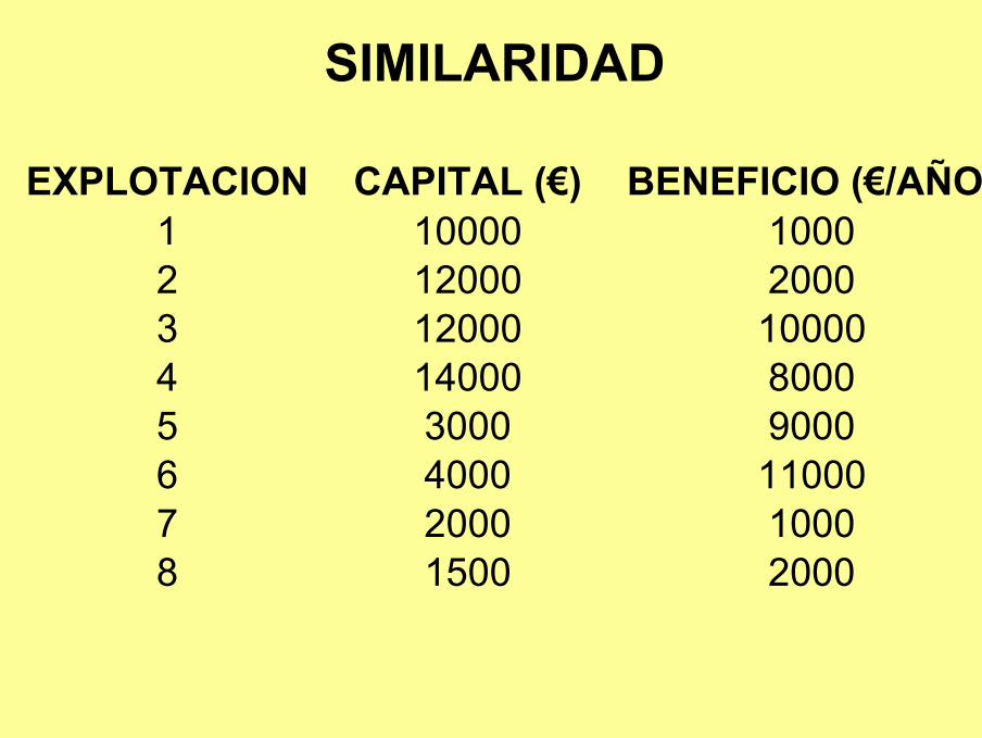
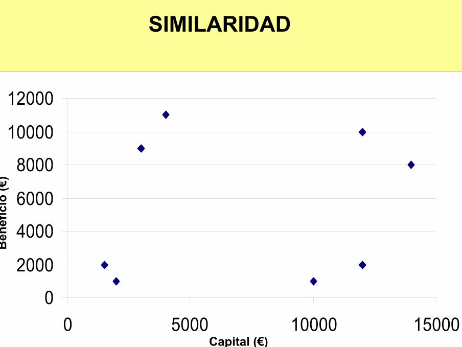
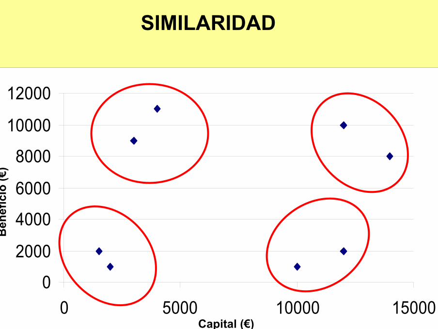
SIMILARIDAD
EXPLOTACION CAPITAL (€) BENEFICIO (€/AÑO)1 10000 10002 12000 20003 12000 100004 14000 80005 3000 90006 4000 110007 2000 10008 1500 2000
SIMILARIDAD
0
2000
4000
6000
8000
10000
12000
0 5000 10000 15000Capital (€)
Ben
efic
io (€
)
SIMILARIDAD
0
2000
4000
6000
8000
10000
12000
0 5000 10000 15000Capital (€)
Ben
efic
io (€
)

SIMILARIDAD
¿Qué se hace cuando k=50?
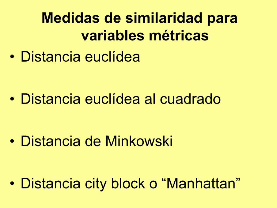
Medidas de similaridad para variables métricas
• Distancia euclídea
• Distancia euclídea al cuadrado
• Distancia de Minkowski
• Distancia city block o “Manhattan”
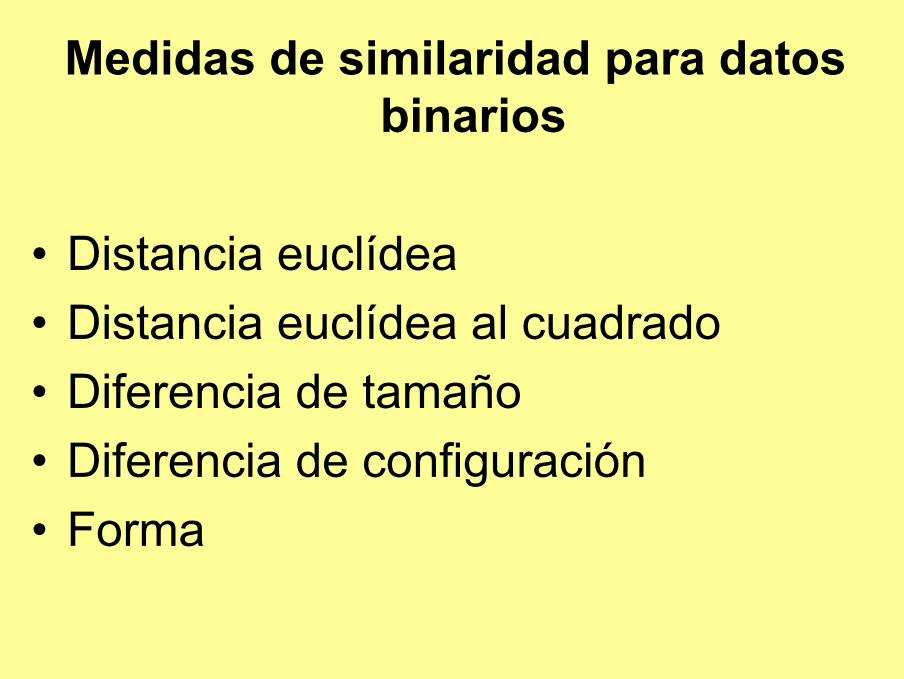
Medidas de similaridad para datos binarios
• Distancia euclídea• Distancia euclídea al cuadrado• Diferencia de tamaño• Diferencia de configuración• Forma
Estandarización de los datos
¿Por qué estandarizar datos?
- Número de animales (n)- Beneficio anual (€/año)- Superficie (ha)

Estandarización de los datos
• Puntuaciones Z: media 0 y DT 1
• Rango 1
• Rango 0 a 1: de 0 a 3
Formación de los grupos
- Algoritmo de agrupación (…)
- Número de grupos razonable (…)

Algoritmo de agrupación
• Análisis jerárquico (10 a 1)
• Análisis no jerárquico (5 a 5)
Análisis jerárquico
• Método del centroide• Método del vecino más cercano• Método del vecino más lejano• Método de la vinculación promedio• Método de Ward
Análisis jerárquico
• Método del centroide
– 2 observaciones cercanas– 1 centroide con valor medio– se repite el proceso

DendrogramCentroid Method,EuclideanD
ista
nce
0
1
2
3
4
5
61 2 345 67 89 10 11 1213 1415 16171819 2021 22 2324 25 2627 28 2930 3132 3334 35 3637 38 3940414243 44 45 46 474849 5051 5253 545556 57 5859606162 6364 65 66 6768 69 7071 7273 74 7576 77 78 7980 81 82838485 86 87 88
Análisis jerárquico
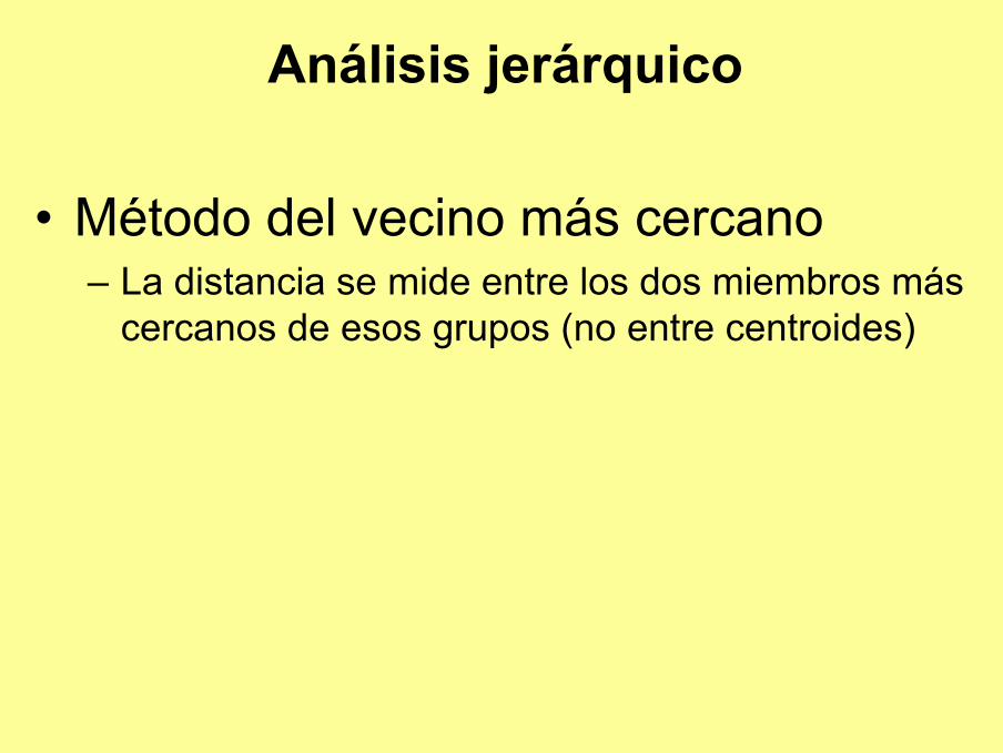
• Método del vecino más cercano– La distancia se mide entre los dos miembros más
cercanos de esos grupos (no entre centroides)
Análisis jerárquico
• Método del vecino más cercano– La distancia se mide entre los dos miembros más
cercanos de esos grupos (no entre centroides)
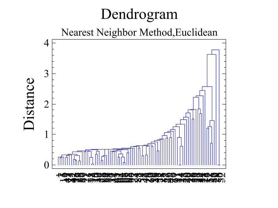
DendrogramNearest Neighbor Method,Euclidean
Dis
tanc
e
0
1
2
3
41 2 345 67 89 10 11 1213 1415 16171819 2021 22 2324 25 2627 28 2930 3132 3334 35 3637 38 3940414243 44 45 46 4748 49 5051 5253 545556 57 58596061 62 6364 65 66 6768 69 7071 7273 74 7576 77 7879 80 81 82838485 86 87 88
Análisis jerárquico
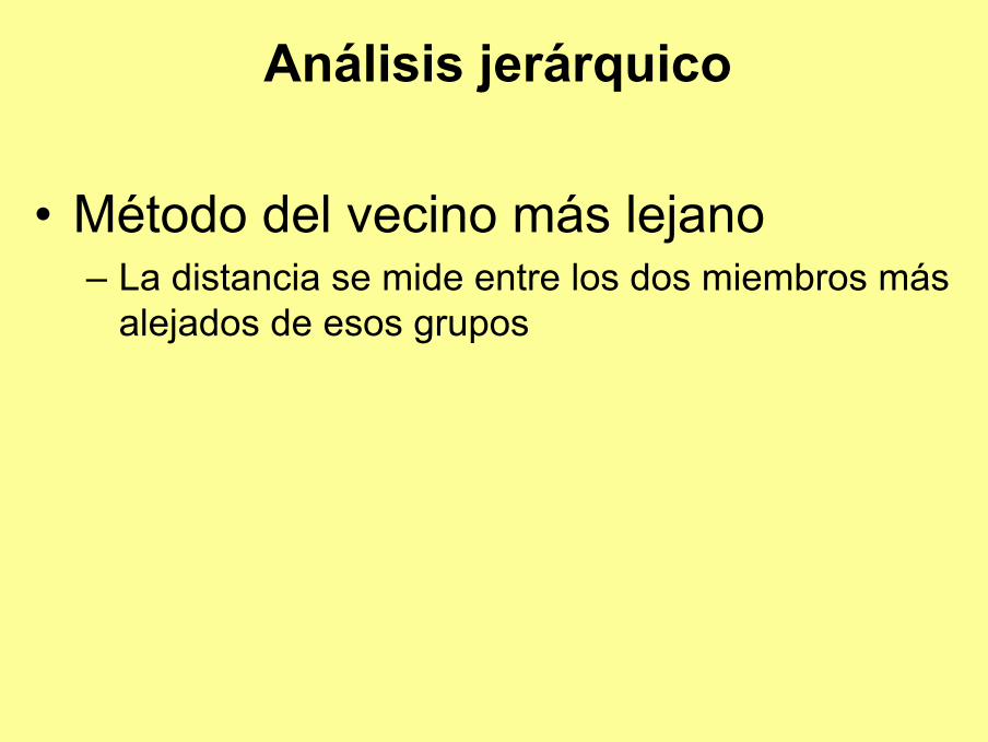
• Método del vecino más lejano– La distancia se mide entre los dos miembros más
alejados de esos grupos

Análisis jerárquico
• Método del vecino más lejano– La distancia se mide entre los dos miembros más
alejados de esos grupos
DendrogramFurthest Neighbor Method,Euclidean
Dis
tanc
e
0
2
4
6
8
101 234 5 67 89 10 11 1213 1415 16171819 2021 22 2324 25 2627 28 2930 3132 3334 35 3637 38 39 404142 43 44 45 46 47 4849 5051 5253 54 5556 57 58 5960 61 6263 6465 66 6768 69 70717273 74 75 76 77 7879 80 81 82838485 86 87 88
Análisis jerárquico
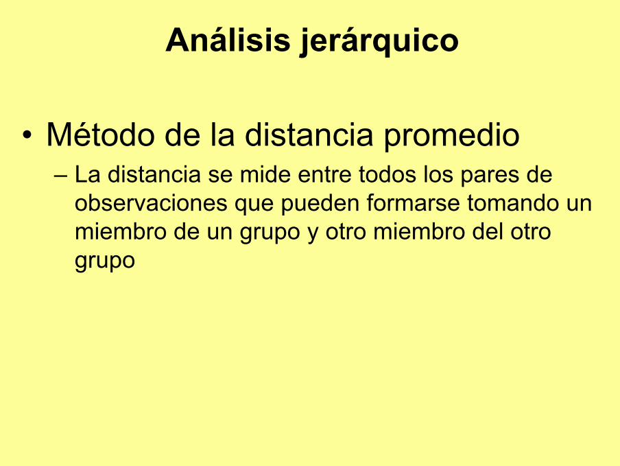
• Método de la distancia promedio– La distancia se mide entre todos los pares de
observaciones que pueden formarse tomando un miembro de un grupo y otro miembro del otro grupo

DendrogramGroup Average Method,Euclidean
Dis
tanc
e
0
2
4
6
81 2 345 67 89 10 11 1213 1415 16171819 2021 22 2324 25 2627 28 2930 3132 3334 35 3637 38 39404142 43 44 45 46 47 4849 5051 5253 54 5556 57 58 5960 61 62 6364 65 66 6768 69 7071 7273 74 7576 77 7879 80 81 82838485 86 87 88
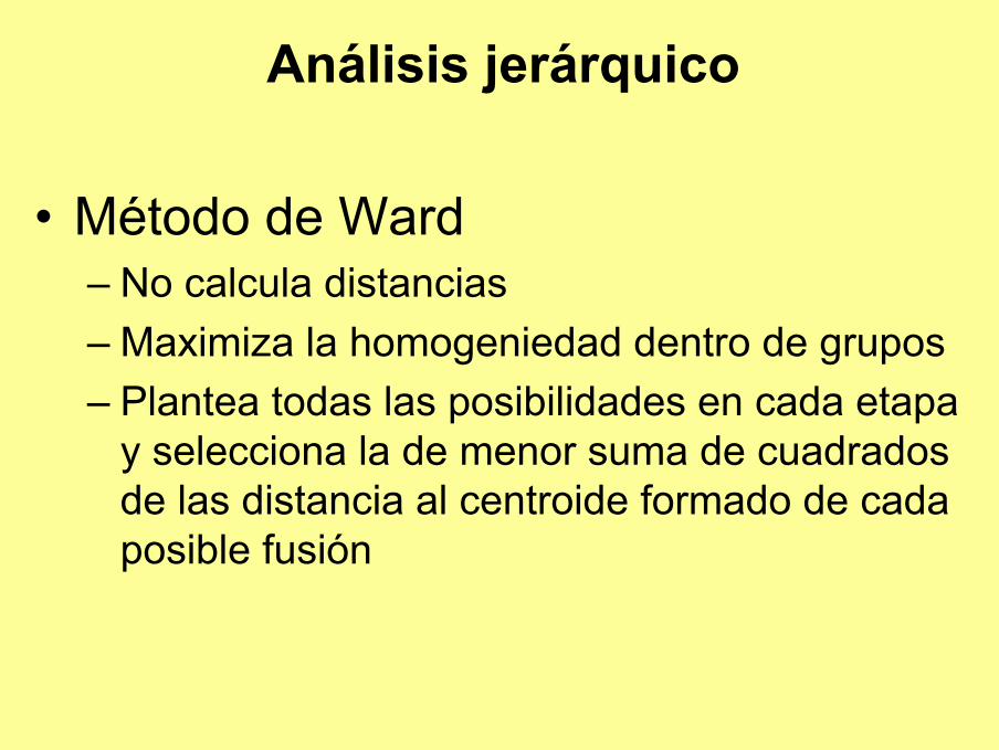
Análisis jerárquico
• Método de Ward– No calcula distancias– Maximiza la homogeniedad dentro de grupos– Plantea todas las posibilidades en cada etapa
y selecciona la de menor suma de cuadrados de las distancia al centroide formado de cada posible fusión
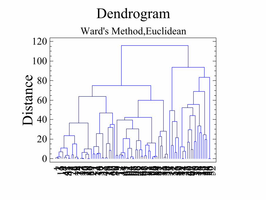
DendrogramWard's Method,Euclidean
Dis
tanc
e
0
20
40
60
80
100
1201 2 34 5 67 89 10 111213 1415 16171819 20 21 22 2324 252627 28 293031 32 3334 353637 38 39404142 43 44 45 46 474849 5051 5253 545556 57 585960 61 62 6364 65 66 6768 69 70717273 74 75 76 77 7879 80 81 8283 8485 86 87 88
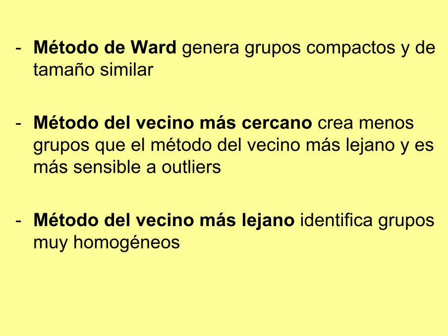
- Método de Ward genera grupos compactos y de tamaño similar
- Método del vecino más cercano crea menos grupos que el método del vecino más lejano y es más sensible a outliers
- Método del vecino más lejano identifica grupos muy homogéneos

Número de grupos
- Distancia. Los grupos a unir están a una distancia mayor de los que ya se han unido
- Tasa de variación. Calcular la tasa de variación entre los coeficientes de conglomeración obtenidos entre etapas sucesivas. Se detiene cuando el incremento en la tasa es drásticamente superior a la anterior.
- Distancia entre conglomerados. Entre centroides.

Número de grupos
- RMS STD es mínima. Suma de las desviaciones típicas de todas las variables que forman el grupo respecto al centroide, cuando se forma un nuevo conglomerado. Indica la homogeneidad entre grupos. (m)
- R2 semiparcial. Indica la pérdida de homogeneidad tras la fusión. (m)
- R2. Ratio entre la heterogeneidad entre grupos y heterogeneidad total, medido como suma de distancias euclideas. (1)

Número de grupos
¿Qué hago?Distancia homogeneidad de los conglomerados fusionados
el valor debe ser pequeño
RMS homogeneidad del nuevo conglomeradoel valor debe ser pequeño
SPR homogeneidad de los conglomerados fusionadosel valor debe ser pequeño
RS heterogeneidad entre conglomeradosel valor debe ser grande (1)
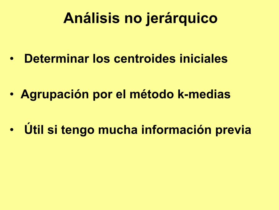
Análisis no jerárquico
• Determinar los centroides iniciales
• Agrupación por el método k-medias
• Útil si tengo mucha información previa

A nivel práctico
¿Jerárquico o no jerárquico?
- Objetivo del estudio- Información previa y habilidad del investigador- Utilizar ambos tipos de modo complementario
A nivel práctico
¿Número de grupos?
- Indicadores anteriores- Dendograma- Experiencia del investigador- Estabilidad de resultados (ANOVA)- Resultados sean razonables y respondan a criterios naturales

Pasos a seguir
1. Estudio jerárquico exploratorio con diferentes métodos de agrupación y distancias; y sucesivos grupos.
2. Determinar la distancia y el método (naturaleza del estudio, número de casos, …)
3. Determinar el número de grupos1. Indicadores anteriores2. Probando el anterior y el siguiente3. ANOVA4. Interpretación de resultados

DOCUMENTOS DE TRABAJO
DPTO PRODUCCION ANIMAL PRODUCCION ANIMAL Y GESTION UNIVERSIDAD DE CORDOBA ISSN: 1698-4226 DT 1, Vol. 1/2004
1
METODOLOGÍA PARA LA CARACTERIZACIÓN Y TIPIFICACIÓN DE
SISTEMAS GANADEROS. 1 Instituto Dominicano de Investigaciones Agropecuarias y Forestales (IDIAF). Republica Dominicana. 2 Profesor de Economía Agraria. Universidad de Córdoba (UCO). España. 3 Profesora del Área de Organización de Empresas. Universidad de Córdoba (UCO). España. 4 Profesor de Producción Animal de la Facultad de Ciencias Veterinarias de la Universidad Nacional de la Pampa (Argentina). 5 Becario del Departamento de Producción Animal. Universidad de Córdoba (UCO). España. 6 Profesor de Estadística, Econometría e Investigación Operativa. Universidad de Córdoba (UCO). España. INTRODUCCIÓN
El alto grado de heterogeneidad que existe entre las explotaciones que conforman una población dificulta la toma de decisiones de carácter transversal. En tal sentido al agrupar las explotaciones de acuerdo a sus principales diferencias y relaciones, se busca maximizar la homogeneidad dentro de los grupos y la heterogeneidad entre los grupos. La metodología de investigación relacionada con los sistemas de producción, tiene como base el conocimiento de los factores (exógenos y endógenos) que intervienen en los mismos, como una necesidad obligada para el desarrollo de alternativas de gestión (Castaldo et al., 2003). Así la planificación de acciones de investigación requiere distinguir los diferentes grupos o tipos que coexisten en la población estudiada, considerando los diversos aspectos en que se desarrollan los sistemas de producción y sus reacciones frente a las evoluciones tecnológicas (Avila 2000). Según Bolaños (1999) la caracterización no es más que la descripción de las características principales y las múltiples interrelaciones de las organizaciones; en tanto que la tipificación se refiere al establecimiento y construcción de grupos posibles basados en las características observadas en la realidad. Para la caracterización y tipificación de los sistemas, se han utilizado diversas técnicas de análisis estadísticos; Mainar et al., (1993) utilizan técnicas de análisis de varianza; Martos et al., (1995), Castaldo et al., (2003) y García et al., (2003) proponen en ganadería extensiva la utilización de técnicas de ANOVA para establecer los factores; mientras que Pardos et al., (1997), Rapey et al., (2001), Sraïri et al.,(2003), Macedo et al., (2003), Castel et al, (2003), Siegmund-Schultze et al., (2001) y Paz et al, (2003), utilizan técnicas de análisis multivariante como el análisis de componentes principales, correspondencia múltiple y análisis cluster, los que incluyen un conjunto de técnicas y métodos que nos permiten estudiar conjuntos de variables en una población de individuos. Finalmente otra parte fundamental de esta metodología es la validación de los resultados obtenidos con la realidad de las explotaciones que conforman la población estudiada. La información obtenida de un estudio de caracterización y tipificación es considerada de gran utilidad a fin de proponer estrategias que permitan mejorar los aspectos que tienen mayor incidencia en el desarrollo de las empresas ganaderas estudiadas.
Daniel Valerio Cabrera1
Antón García Martínez2
Raquel Acero de la Cruz3 Ariel Castaldo 4
José Manuel Perea5 José Martos Peinado6
DOCUMENTOS DE TRABAJO
DPTO PRODUCCION ANIMAL PRODUCCION ANIMAL Y GESTION UNIVERSIDAD DE CORDOBA ISSN: 1698-4226 DT 1, Vol. 1/2004
2
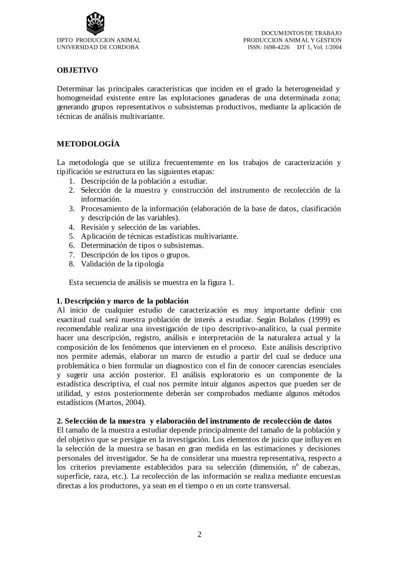
OBJETIVO Determinar las principales características que inciden en el grado la heterogeneidad y homogeneidad existente entre las explotaciones ganaderas de una determinada zona; generando grupos representativos o subsistemas productivos, mediante la aplicación de técnicas de análisis multivariante. METODOLOGÍA La metodología que se utiliza frecuentemente en los trabajos de caracterización y tipificación se estructura en las siguientes etapas:
1. Descripción de la población a estudiar. 2. Selección de la muestra y construcción del instrumento de recolección de la
información. 3. Procesamiento de la información (elaboración de la base de datos, clasificación
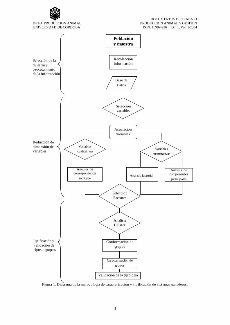
y descripción de las variables). 4. Revisión y selección de las variables. 5. Aplicación de técnicas estadísticas multivariante. 6. Determinación de tipos o subsistemas. 7. Descripción de los tipos o grupos. 8. Validación de la tipología Esta secuencia de análisis se muestra en la figura 1.
1. Descripción y marco de la población Al inicio de cualquier estudio de caracterización es muy importante definir con exactitud cual será nuestra población de interés a estudiar. Según Bolaños (1999) es recomendable realizar una investigación de tipo descriptivo-analítico, la cual permite hacer una descripción, registro, análisis e interpretación de la naturaleza actual y la composición de los fenómenos que intervienen en el proceso. Este análisis descriptivo nos permite además, elaborar un marco de estudio a partir del cual se deduce una problemática o bien formular un diagnostico con el fin de conocer carencias esenciales y sugerir una acción posterior. El análisis exploratorio es un componente de la estadística descriptiva, el cual nos permite intuir algunos aspectos que pueden ser de utilidad, y estos posteriormente deberán ser comprobados mediante algunos métodos estadísticos (Martos, 2004). 2. Selección de la muestra y elaboración del instrumento de recolección de datos El tamaño de la muestra a estudiar depende principalmente del tamaño de la población y del objetivo que se persigue en la investigación. Los elementos de juicio que influyen en la selección de la muestra se basan en gran medida en las estimaciones y decisiones personales del investigador. Se ha de considerar una muestra representativa, respecto a los criterios previamente establecidos para su selección (dimensión, no de cabezas, superficie, raza, etc.). La recolección de las información se realiza mediante encuestas directas a los productores, ya sean en el tiempo o en un corte transversal.
DOCUMENTOS DE TRABAJO
DPTO PRODUCCION ANIMAL PRODUCCION ANIMAL Y GESTION UNIVERSIDAD DE CORDOBA ISSN: 1698-4226 DT 1, Vol. 1/2004
3
Selección de la muestra y procesamiento de la información Reducción de dimensión de variables Tipificación y validación de tipos o grupos
Figura 1. Diagrama de la metodología de caracterización y tipificación de sistemas ganaderos.
Población y muestra
Recolección información
Base de Datos
Selección variables
Asociación variables
Variables cualitativas
Variables cuantitativas
Selección Factores
Análisis Cluster
Conformación de grupos
Caracterización de grupos
Validación de la tipología
Análisis de correspondencia
múltiple
Análisis factorial
Análisis de componentes principales
DOCUMENTOS DE TRABAJO
DPTO PRODUCCION ANIMAL PRODUCCION ANIMAL Y GESTION UNIVERSIDAD DE CORDOBA ISSN: 1698-4226 DT 1, Vol. 1/2004
4
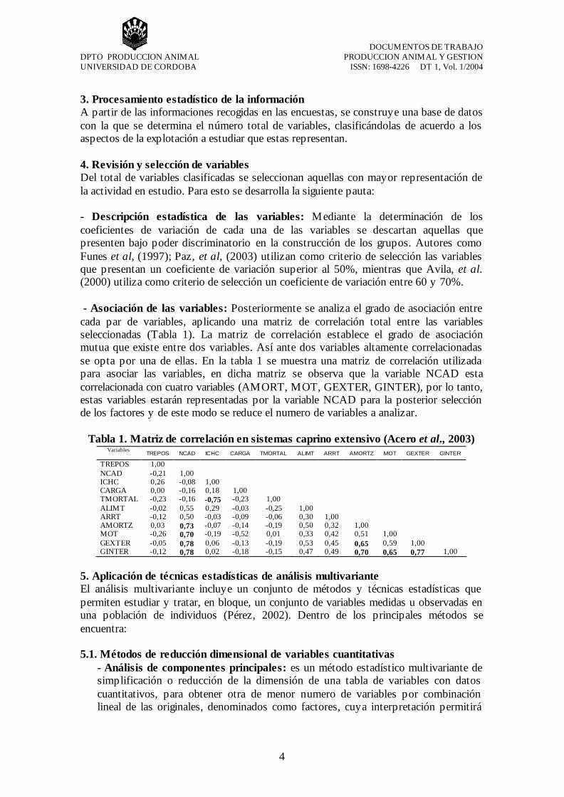
3. Procesamiento estadístico de la información A partir de las informaciones recogidas en las encuestas, se construye una base de datos con la que se determina el número total de variables, clasificándolas de acuerdo a los aspectos de la explotación a estudiar que estas representan. 4. Revisión y selección de variables Del total de variables clasificadas se seleccionan aquellas con mayor representación de la actividad en estudio. Para esto se desarrolla la siguiente pauta: - Descripción estadística de las variables: Mediante la determinación de los coeficientes de variación de cada una de las variables se descartan aquellas que presenten bajo poder discriminatorio en la construcción de los grupos. Autores como Funes et al, (1997); Paz, et al, (2003) utilizan como criterio de selección las variables que presentan un coeficiente de variación superior al 50%, mientras que Avila, et al. (2000) utiliza como criterio de selección un coeficiente de variación entre 60 y 70%. - Asociación de las variables: Posteriormente se analiza el grado de asociación entre cada par de variables, aplicando una matriz de correlación total entre las variables seleccionadas (Tabla 1). La matriz de correlación establece el grado de asociación mutua que existe entre dos variables. Así ante dos variables altamente correlacionadas se opta por una de ellas. En la tabla 1 se muestra una matriz de correlación utilizada para asociar las variables, en dicha matriz se observa que la variable NCAD esta correlacionada con cuatro variables (AMORT, MOT, GEXTER, GINTER), por lo tanto, estas variables estarán representadas por la variable NCAD para la posterior selección de los factores y de este modo se reduce el numero de variables a analizar.
Tabla 1. Matriz de correlación en sistemas caprino extensivo (Acero et al., 2003)
Variables TREPOS NCAD ICHC CARGA TMORTAL ALIMT ARRT AMORTZ MOT GEXTER GINTER
TREPOS NCAD ICHC CARGA TMORTAL ALIMT ARRT AMORTZ MOT GEXTER GINTER
1,00 -0,21 0,26 0,00 -0,23 -0,02 -0,12 0,03 -0,26 -0,05 -0,12
1,00 -0,08 -0,16 -0,16 0,55 0,50 0,73 0,70 0,78 0,78
1,00 0,18 -0,75 0,29 -0,03 -0,07 -0,19 0,06 0,02
1,00 -0,23 -0,03 -0,09 -0,14 -0,52 -0,13 -0,18
1,00 -0,25 -0,06 -0,19 0,01 -0,19 -0,15
1,00 0,30 0,50 0,33 0,53 0,47
1,00 0,32 0,42 0,45 0,49
1,00 0,51 0,65 0,70
1,00 0,59 0,65
1,00 0,77
1,00
5. Aplicación de técnicas estadísticas de análisis multivariante El análisis multivariante incluye un conjunto de métodos y técnicas estadísticas que permiten estudiar y tratar, en bloque, un conjunto de variables medidas u observadas en una población de individuos (Pérez, 2002). Dentro de los principales métodos se encuentra: 5.1. Métodos de reducción dimensional de variables cuantitativas
- Análisis de componentes principales: es un método estadístico multivariante de simplificación o reducción de la dimensión de una tabla de variables con datos cuantitativos, para obtener otra de menor numero de variables por combinación lineal de las originales, denominados como factores, cuya interpretación permitirá
DOCUMENTOS DE TRABAJO
DPTO PRODUCCION ANIMAL PRODUCCION ANIMAL Y GESTION UNIVERSIDAD DE CORDOBA ISSN: 1698-4226 DT 1, Vol. 1/2004
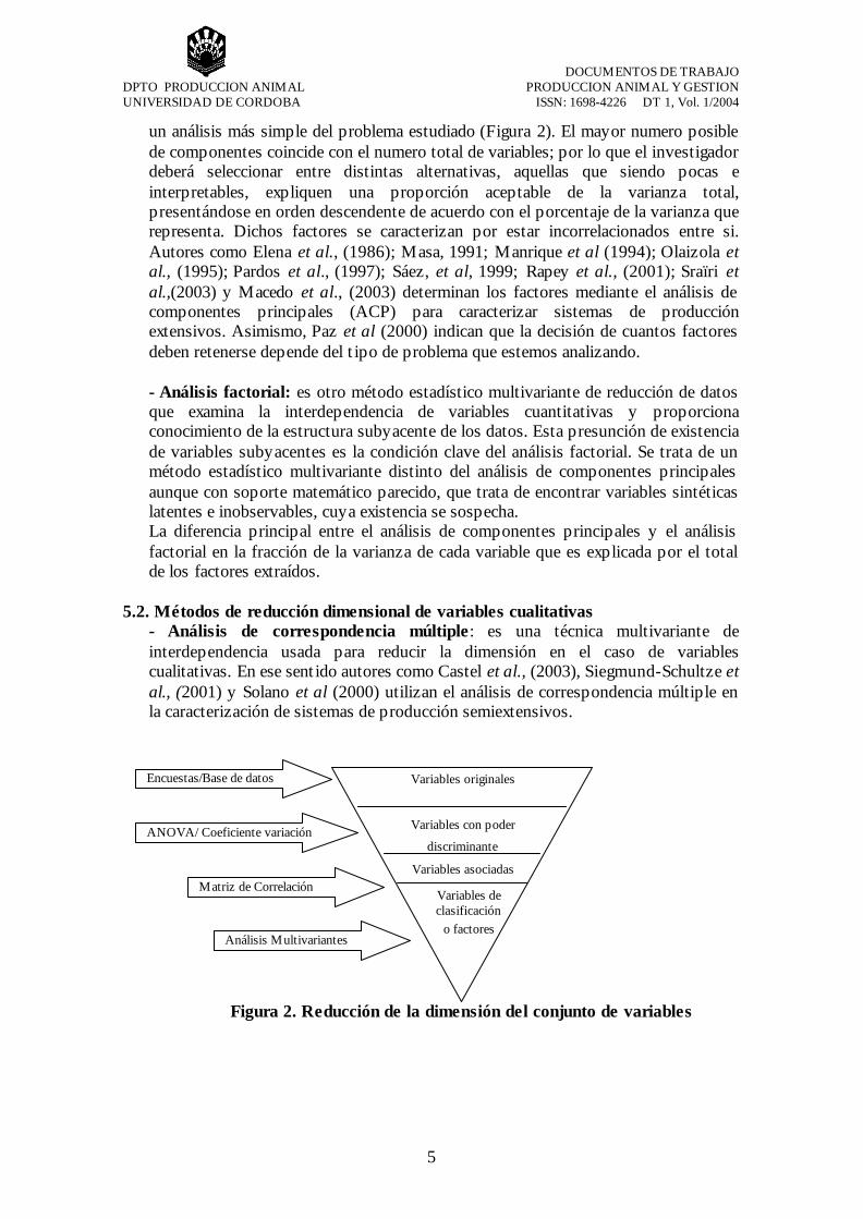
5
un análisis más simple del problema estudiado (Figura 2). El mayor numero posible de componentes coincide con el numero total de variables; por lo que el investigador deberá seleccionar entre distintas alternativas, aquellas que siendo pocas e interpretables, expliquen una proporción aceptable de la varianza total, presentándose en orden descendente de acuerdo con el porcentaje de la varianza que representa. Dichos factores se caracterizan por estar incorrelacionados entre si. Autores como Elena et al., (1986); Masa, 1991; Manrique et al (1994); Olaizola et al., (1995); Pardos et al., (1997); Sáez, et al, 1999; Rapey et al., (2001); Sraïri et al.,(2003) y Macedo et al., (2003) determinan los factores mediante el análisis de componentes principales (ACP) para caracterizar sistemas de producción extensivos. Asimismo, Paz et al (2000) indican que la decisión de cuantos factores deben retenerse depende del tipo de problema que estemos analizando. - Análisis factorial: es otro método estadístico multivariante de reducción de datos que examina la interdependencia de variables cuantitativas y proporciona conocimiento de la estructura subyacente de los datos. Esta presunción de existencia de variables subyacentes es la condición clave del análisis factorial. Se trata de un método estadístico multivariante distinto del análisis de componentes principales aunque con soporte matemático parecido, que trata de encontrar variables sintéticas latentes e inobservables, cuya existencia se sospecha. La diferencia principal entre el análisis de componentes principales y el análisis factorial en la fracción de la varianza de cada variable que es explicada por el total de los factores extraídos.
5.2. Métodos de reducción dimensional de variables cualitativas
- Análisis de correspondencia múltiple: es una técnica multivariante de interdependencia usada para reducir la dimensión en el caso de variables cualitativas. En ese sentido autores como Castel et al., (2003), Siegmund-Schultze et al., (2001) y Solano et al (2000) utilizan el análisis de correspondencia múltiple en la caracterización de sistemas de producción semiextensivos.
Figura 2. Reducción de la dimensión del conjunto de variables
Variables originales
Variables con poder
discriminante
Variables asociadas
Variables de clasificación
o factores
Encuestas/Base de datos
ANOVA/ Coeficiente variación
Matriz de Correlación
Análisis Multivariantes

DOCUMENTOS DE TRABAJO
DPTO PRODUCCION ANIMAL PRODUCCION ANIMAL Y GESTION UNIVERSIDAD DE CORDOBA ISSN: 1698-4226 DT 1, Vol. 1/2004
6
6. Determinación de Tipos o subsistemas productivos - Análisis Cluster (Conglomerados) Una vez concretados y seleccionados los factores se procede al análisis multivariante cluster, el cual es un método estadístico de clasificación de datos, que permite establecer grupos homogéneos de explotaciones a la vez que heterogéneos entre los mismos. Autores como Mainar, et al, (1993); Sáez et al, (1997); Castel et al, (2000); Siegmund-Schultze et al., (2001); Macedo et al., (2003); Solano et al. (2003); Sraïri et al.,(2003) lo utilizan para clasificar y agrupar sistemas productivos extensivos y semiextensivos. Existen dos grandes tipos de análisis cluster: aquellos que asignan los casos a grupos diferenciados que el propio análisis configura, sin que unos dependan de otros, se conocen como no jerárquicos. Existen otros que configuran grupos con estructuras arborescentes, de forma que cluster de niveles más bajos van siendo englobados en otros de niveles superiores, se denominan jerárquicos (Pérez, 2002). El resultado del análisis cluster normalmente se expresa gráficamente en un diagrama de árbol o dendograma (figura 2). - Análisis Discriminante Esta técnica estadística permite asignar o clasificar nuevos individuos dentro de grupos previamente definidos; por lo tanto solo será aplicada cuando se considere necesario, posteriormente a la tipificación de las explotaciones.
DendrogramaWard's Method,Squared Euclidean
Dis
tanc
ia
0
10
20
30
40
1 5 9 14 1822 2630 3640 4448 52 56
Figura 2. Dendograma de clasificación de explotaciones en tres subsistemas
7. Determinación y descripción de los tipos seleccionados A partir del dendograma el investigador observara el nivel que aparezca como representativo desde el punto de vista del número de grupos resultantes, tomando en cuenta que se cumpla el criterio de máxima homogeneidad dentro de los grupos y máxima heterogeneidad entre grupos. La descripción de los grupos se realiza mediante el calculo de medidas de situación en la estadística descriptiva (media, mediana, moda, etc.) al conjunto de variables originales para cada tipo o grupo determinado.
DOCUMENTOS DE TRABAJO
DPTO PRODUCCION ANIMAL PRODUCCION ANIMAL Y GESTION UNIVERSIDAD DE CORDOBA ISSN: 1698-4226 DT 1, Vol. 1/2004
7
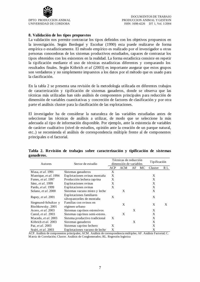
8. Validación de los tipos propuestos La validación nos permite contrastar los tipos definidos con los objetivos propuestos en la investigación. Según Berdegué y Escobar (1990) esta puede realizarse de forma empírica o estadísticamente. El método empírico es realizado por el investigador u otras personas conocedoras de los sistemas productivos estudiados, capaces de contrastar los tipos obtenidos con los existentes en la realidad. La forma estadística consiste en repetir la tipificación mediante el uso de técnicas estadísticas diferentes y comparando los resultados finales. Según Köbrich et al (2003) es importante asegurar que estos grupos son verdaderos y no simplemente impuestos a los datos por el método que es usado para la clasificación. En la tabla 2 se presenta una revisión de la metodología utilizada en diferentes trabajos de caracterización y tipificación de sistemas ganaderos, donde se observa que las técnicas más utilizadas han sido análisis de componentes principales para reducción de dimensión de variables cuantitativas y concreción de factores de clasificación y por otra parte el análisis cluster para la clasificación de las explotaciones. El investigador ha de considerar la naturaleza de las variables estudiadas antes de seleccionar las técnicas de análisis a utilizar, de modo que se seleccione la más adecuada al tipo de información disponible. Por ejemplo, ante la existencia de variables de carácter cualitativo (nivel de estudios, opinión ante la creación de un parque natural, etc..) se recomienda el análisis de correspondencia múltiple frente al de componentes principales o el factorial. Tabla 2. Revisión de trabajos sobre caracterización y tipificación de sistemas ganaderos.
Técnicas de reducción dimensión de variables Tipificación Autores Sector de estudio
ACP ACM AF MC Cluster R L Masa, et al. 1991 Sistemas ganaderos X Manrique, et al. 1994 Explotaciones ovinas montaña X X Funes, et al. 1997 Producción lechera caprina X X Sáez, et al. 1999 Explotaciones ovinas X X Pardo, et al. 1999 Explotaciones ovinas X X Solano, et al. 2000 Sistemas vacuno mixto y leche X X
Rapey, et al. 2001 Explotaciones familiares silvopastoriles de montaña X X
Siegmund-Schultze y Rischkowsky. 2001
Familias con ovinos en régimen urbano X X X
Acero, et al. 2003 Sistemas caprinos extensivos X X Castel, et al. 2003 Sistemas caprinos semi-extens. X X Macedo, et al. 2003 Sistema productivo tradicional X X Köbrich et al. 2003 Sistemas ganaderos X X Paz, et al. 2003 Sistemas caprino lechero X X Sraïri, et al. 2003 Explotaciones vacuno de leche X X
ACP. Análisis de componentes principales; ACM. Análisis de correspondencia múltiples; AF. Análisis Factorial; C. Matriz de Correlación; Cluster. Análisis de Conglomerados; RL. Regresión logística
DOCUMENTOS DE TRABAJO
DPTO PRODUCCION ANIMAL PRODUCCION ANIMAL Y GESTION UNIVERSIDAD DE CORDOBA ISSN: 1698-4226 DT 1, Vol. 1/2004
8
CONCLUSIONES Los estudios de caracterización y tipificación nos permiten realizar una mejor planificación y distribución más eficiente de los recursos destinados a mejorar el funcionamiento de los diferentes sistemas productivos que conforman el entorno de la población estudiada. Para realizar un estudio de caracterización y tipificación existen una gran diversidad de técnicas, de las cuales el investigador debe seleccionar aquellas que considere más adecuadas a sus datos y sobre todo a su objetivo científico. REFERENCIAS Álvarez, R., Paz, R. 1997. Metodología asociada al diseño de propuestas para el
desarrollo de la producción lechera caprina. Archivos de Zootecnia. Vol 46. Nº 175. Pag. 211-222.
Avila, L., Muños, M., Rivera, B. 2000. Tipificación de los sistemas de producción agropecuaria en la zona de influencia del programa UNIR (CALDAS). Universidad de Caldas, Departamento de sistemas de producción, Programa UNIR.
Berdegué, J. y Escobar, G. 1990. Metodología para la tipificación de sistemas de finca. RIMISP. Santiago de Chile. Pag. 13-43.
Bolaños, O. 1999. Caracterización y tipificación de organizaciones de productores y productoras. Unidad de planificación estratégica. Ministerio de agricultura y ganadería. XI Congreso Nacional Agronómico / I Congreso Nacional de Extensión. Costa Rica.
Castaldo, A., Acero de la Cruz, R., García Martínez, A., Martos, J., Pamio, J., Mendoza García, F. 2003. Caracterización de la invernada en el nordeste de la provincia de La Pampa (Argentina). XXIV Reunión Anual de la Asociación argentina de Economía Agraria. Río Cuarto. Argentina.
Castel, J. M., Mena, Y., Delgado-Pertínez, M., Camúñez, J., Basulto, J., Caravaca, F., Guzmán-Guerrero, J.L., Alcalde, M.J. 2003. Characterization of semi-extensive goat production systems in southern Spain. Small Ruminant Research. Nº 47. Pág. 133-143.
Elena Rosello, M.; Cornut, E., López Marquez, J.A. 1986. Estructura del sistema productivo del ecosistema de dehesa. Servicio de extensión y capacitación agraria. Badajoz. España.
Acero, R., Martos, J., García, A., Luque, M., Herrera, M., Peña, F. 2003. Characterization of extensive goat systems through factorial analysis. International Symposium. Animal Production and natural resources utilization in the Mediterranean Mountain Areas. Grecia.
Macedo, R., Galina, M.A., Zorrilla, J.M., Palma, J.M., Pérez Guerrero, J. 2003. Análisis de un sistema de producción tradicional en Colima, México. Archivos de Zootecnia. Vol 52. Nº 200. Pag. 463-474.
Mainar, R.C., Cuesta, P., Méndez, I., Asensio, M.A., Domínguez, L., Vázquez-Boland, J.A. 1993. Caracterización de la explotación ovina y caprina de la C.A.M.

DOCUMENTOS DE TRABAJO
DPTO PRODUCCION ANIMAL PRODUCCION ANIMAL Y GESTION UNIVERSIDAD DE CORDOBA ISSN: 1698-4226 DT 1, Vol. 1/2004
9
mediante encuestas y análisis multivariante: Bases para una planificación en ganadería y sanidad animal. SEOC XIX.
Manrique, E., Maza, M. T., Olaizola, A. 1992. Classification systems in livestock farming: how and why? The point of view of a production economist. In II International Symposium the study of livestock farming systems in a research and development framework. Zaragoza. 5 pp.
Martos Peinado, J., García Martínez, A., Rodríguez Alcaide, J.J. y Acero de la Cruz, R. 1995. Clasificación técnico económica de las explotaciones lácteas de la Campiña Baja Cordobesa. Archivos de Zootecnia. Vol 44. Nº 165. Pág 39-48.
Martos Peinado, J. 2004. Estadística: Conceptos, Práctica Aplicada y Ejercicios. Departamento de Estadística y Organización de Empresas, Universidad de Córdoba, España.
Olaizola, A., Manrique, E., Maza, Mª. 1995. Tipos de sistemas de producción y rendimientos económicos en explotaciones de vacunos de montaña. Información Técnica económica agraria. Vol. 91ª Nº 2. Pág. 47-58.
Pardos Castillo, L., Sáez Olivito, E., González Santos, J.M., Allueva Pinilla, A. 1999. Caracterización técnica de explotaciones ovinas aragonesas mediante métodos estadísticos multivariantes. SEOC. XXII.
Paz, R., Lipshitz, H., Álvarez, R., Usandivaras, P. 2003. Diversidad y Análisis económico en los sistemas de producción lecheros caprinos en el área de riego del Río Dulce-Santiago del Estero-Argentina. ITEA Vol. 99 A Nº 1. Pág. 10-40.
Pérez, C. 2002. Estadística Practica con Statgraphics. Universidad Complutense de Madrid. Editorial Pearson Educación, S. A. Madrid.
Rapey, H., Lifran, R. Valadier, A. 2001. Identifying social, economic and technical determinants of silvopastoral practices in temperate uplands: results of a survey in the Massif central region of France. Agricultural Systems Nº 69. Pág. 119-135.
Sáez Olivito, E., Pardos Castillo, L., González Santos, J. M., Allueva Pinilla, A. 1999. Caracterización estructural de explotaciones ovinas aragonesas mediante métodos estadísticos multivariantes. SEOC XXII.
Siegmund-Schultze, M., Rischkowsky, B. 2001. relating household characteristics to urban sheep keeping in West Africa. Agrycultural Systems Nº 67. Pág. 139-152.
Solano, C., Bernués, A., Rojas, F., Joaquín, N., Fernández, W., Herrero, M. 2000. Relationships between management intensity and structural and social variables in dairy and dual-purpose systems in Santa Cruz, Bolivia. Agricultural Systems Nº 65. Pág. 159-177.
Solano, C., León, H., Pérez, E., Herrero, M. 2003. The role personal information sources on the decision-making process of Costa Rica dairy farmers. Agricultural Systems Nº 76. Pág. 3-18.
Sraïri, M. T., Lyoubi, R. 2003. Typology of dairy farming systems in Rabat Suburban region, Morocco. Archivos de zootecnia Nº 52. Pág. 47-58.
1
Identifying representative farms for determining generic optimal farm management strategies post CAP reform: An application in Northern Ireland.
P. Keatley and D. Anderson
Department of Agricultural and Food Economics, Queen’s University Belfast, Agricultural and Food Science Centre, Newforge Lane, Belfast, BT9 5PX
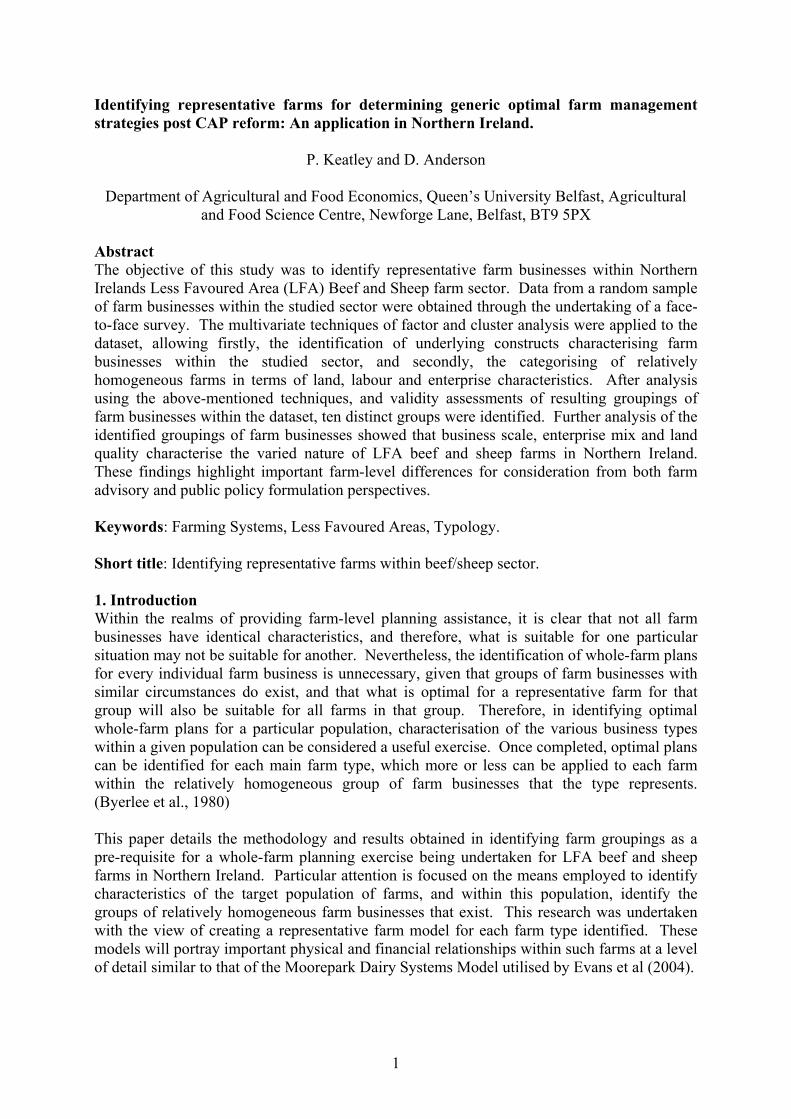
Abstract The objective of this study was to identify representative farm businesses within Northern Irelands Less Favoured Area (LFA) Beef and Sheep farm sector. Data from a random sample of farm businesses within the studied sector were obtained through the undertaking of a face-to-face survey. The multivariate techniques of factor and cluster analysis were applied to the dataset, allowing firstly, the identification of underlying constructs characterising farm businesses within the studied sector, and secondly, the categorising of relatively homogeneous farms in terms of land, labour and enterprise characteristics. After analysis using the above-mentioned techniques, and validity assessments of resulting groupings of farm businesses within the dataset, ten distinct groups were identified. Further analysis of the identified groupings of farm businesses showed that business scale, enterprise mix and land quality characterise the varied nature of LFA beef and sheep farms in Northern Ireland. These findings highlight important farm-level differences for consideration from both farm advisory and public policy formulation perspectives. Keywords: Farming Systems, Less Favoured Areas, Typology. Short title: Identifying representative farms within beef/sheep sector. 1. Introduction Within the realms of providing farm-level planning assistance, it is clear that not all farm businesses have identical characteristics, and therefore, what is suitable for one particular situation may not be suitable for another. Nevertheless, the identification of whole-farm plans for every individual farm business is unnecessary, given that groups of farm businesses with similar circumstances do exist, and that what is optimal for a representative farm for that group will also be suitable for all farms in that group. Therefore, in identifying optimal whole-farm plans for a particular population, characterisation of the various business types within a given population can be considered a useful exercise. Once completed, optimal plans can be identified for each main farm type, which more or less can be applied to each farm within the relatively homogeneous group of farm businesses that the type represents. (Byerlee et al., 1980) This paper details the methodology and results obtained in identifying farm groupings as a pre-requisite for a whole-farm planning exercise being undertaken for LFA beef and sheep farms in Northern Ireland. Particular attention is focused on the means employed to identify characteristics of the target population of farms, and within this population, identify the groups of relatively homogeneous farm businesses that exist. This research was undertaken with the view of creating a representative farm model for each farm type identified. These models will portray important physical and financial relationships within such farms at a level of detail similar to that of the Moorepark Dairy Systems Model utilised by Evans et al (2004).
2
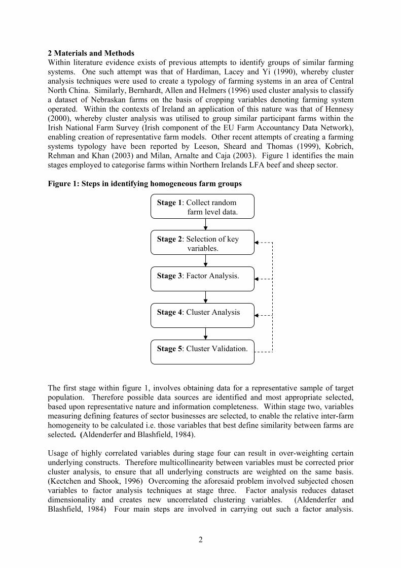
2 Materials and Methods Within literature evidence exists of previous attempts to identify groups of similar farming systems. One such attempt was that of Hardiman, Lacey and Yi (1990), whereby cluster analysis techniques were used to create a typology of farming systems in an area of Central North China. Similarly, Bernhardt, Allen and Helmers (1996) used cluster analysis to classify a dataset of Nebraskan farms on the basis of cropping variables denoting farming system operated. Within the contexts of Ireland an application of this nature was that of Hennesy (2000), whereby cluster analysis was utilised to group similar participant farms within the Irish National Farm Survey (Irish component of the EU Farm Accountancy Data Network), enabling creation of representative farm models. Other recent attempts of creating a farming systems typology have been reported by Leeson, Sheard and Thomas (1999), Kobrich, Rehman and Khan (2003) and Milan, Arnalte and Caja (2003). Figure 1 identifies the main stages employed to categorise farms within Northern Irelands LFA beef and sheep sector. Figure 1: Steps in identifying homogeneous farm groups
The first stage within figure 1, involves obtaining data for a representative sample of target population. Therefore possible data sources are identified and most appropriate selected, based upon representative nature and information completeness. Within stage two, variables measuring defining features of sector businesses are selected, to enable the relative inter-farm homogeneity to be calculated i.e. those variables that best define similarity between farms are selected. (Aldenderfer and Blashfield, 1984). Usage of highly correlated variables during stage four can result in over-weighting certain underlying constructs. Therefore multicollinearity between variables must be corrected prior cluster analysis, to ensure that all underlying constructs are weighted on the same basis. (Kectchen and Shook, 1996) Overcoming the aforesaid problem involved subjected chosen variables to factor analysis techniques at stage three. Factor analysis reduces dataset dimensionality and creates new uncorrelated clustering variables. (Aldenderfer and Blashfield, 1984) Four main steps are involved in carrying out such a factor analysis.
Stage 1: Collect random farm level data.
Stage 2: Selection of key variables.
Stage 3: Factor Analysis.
Stage 4: Cluster Analysis
Stage 5: Cluster Validation.
3
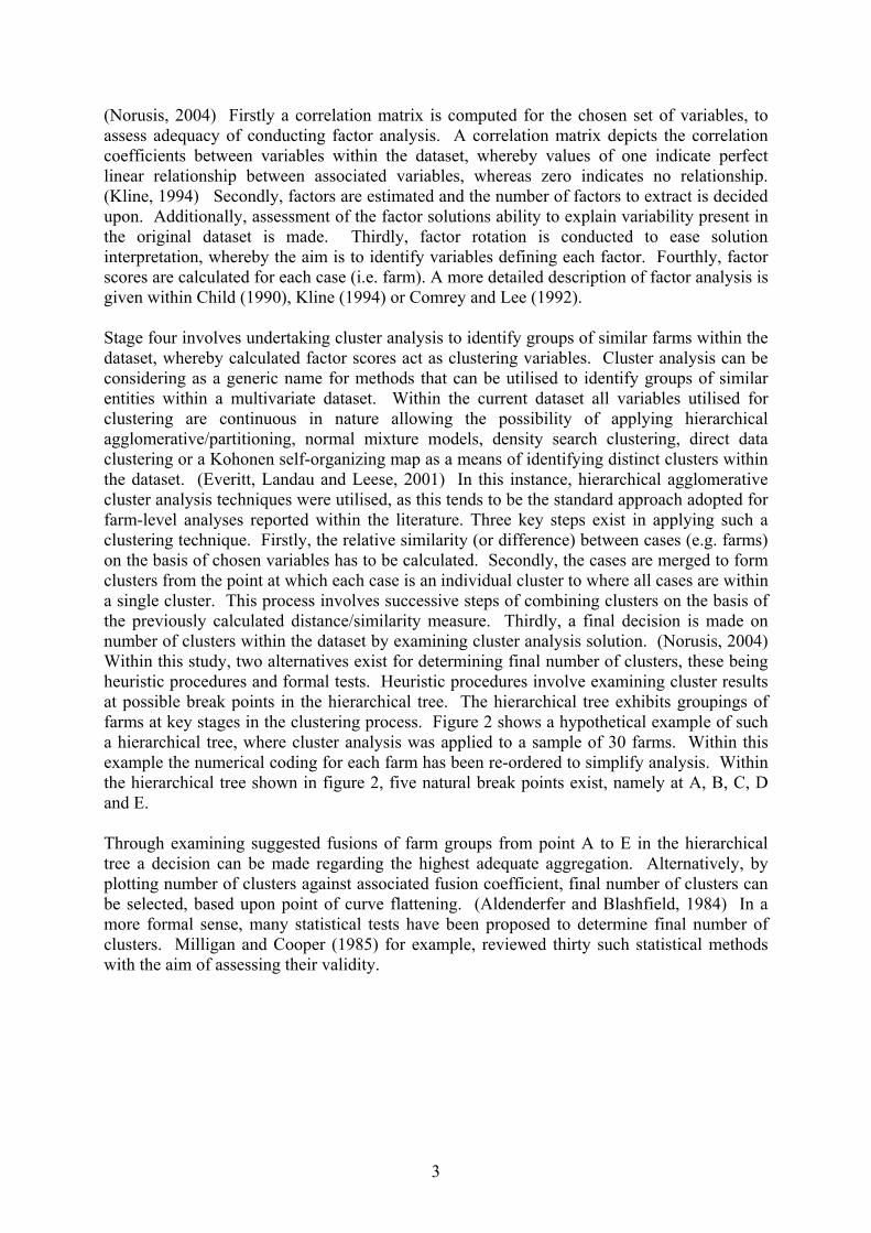
(Norusis, 2004) Firstly a correlation matrix is computed for the chosen set of variables, to assess adequacy of conducting factor analysis. A correlation matrix depicts the correlation coefficients between variables within the dataset, whereby values of one indicate perfect linear relationship between associated variables, whereas zero indicates no relationship. (Kline, 1994) Secondly, factors are estimated and the number of factors to extract is decided upon. Additionally, assessment of the factor solutions ability to explain variability present in the original dataset is made. Thirdly, factor rotation is conducted to ease solution interpretation, whereby the aim is to identify variables defining each factor. Fourthly, factor scores are calculated for each case (i.e. farm). A more detailed description of factor analysis is given within Child (1990), Kline (1994) or Comrey and Lee (1992). Stage four involves undertaking cluster analysis to identify groups of similar farms within the dataset, whereby calculated factor scores act as clustering variables. Cluster analysis can be considering as a generic name for methods that can be utilised to identify groups of similar entities within a multivariate dataset. Within the current dataset all variables utilised for clustering are continuous in nature allowing the possibility of applying hierarchical agglomerative/partitioning, normal mixture models, density search clustering, direct data clustering or a Kohonen self-organizing map as a means of identifying distinct clusters within the dataset. (Everitt, Landau and Leese, 2001) In this instance, hierarchical agglomerative cluster analysis techniques were utilised, as this tends to be the standard approach adopted for farm-level analyses reported within the literature. Three key steps exist in applying such a clustering technique. Firstly, the relative similarity (or difference) between cases (e.g. farms) on the basis of chosen variables has to be calculated. Secondly, the cases are merged to form clusters from the point at which each case is an individual cluster to where all cases are within a single cluster. This process involves successive steps of combining clusters on the basis of the previously calculated distance/similarity measure. Thirdly, a final decision is made on number of clusters within the dataset by examining cluster analysis solution. (Norusis, 2004) Within this study, two alternatives exist for determining final number of clusters, these being heuristic procedures and formal tests. Heuristic procedures involve examining cluster results at possible break points in the hierarchical tree. The hierarchical tree exhibits groupings of farms at key stages in the clustering process. Figure 2 shows a hypothetical example of such a hierarchical tree, where cluster analysis was applied to a sample of 30 farms. Within this example the numerical coding for each farm has been re-ordered to simplify analysis. Within the hierarchical tree shown in figure 2, five natural break points exist, namely at A, B, C, D and E. Through examining suggested fusions of farm groups from point A to E in the hierarchical tree a decision can be made regarding the highest adequate aggregation. Alternatively, by plotting number of clusters against associated fusion coefficient, final number of clusters can be selected, based upon point of curve flattening. (Aldenderfer and Blashfield, 1984) In a more formal sense, many statistical tests have been proposed to determine final number of clusters. Milligan and Cooper (1985) for example, reviewed thirty such statistical methods with the aim of assessing their validity.

4
Figure 2: Dendrogram for a sample of 30 farms Farms 1 2 3 4 5 6 7 8 9 10 11 12 13 14 15 16 17 18 19 20 21 22 23 24 25 26 27 28 29 30
A B C D E Within stage five, validity of final partitions within dataset (i.e. clusters of farm businesses) is assessed. Within this, no techniques are available to guarantee the validity or significance of the cluster solution. (Hair et al, 1998) Nevertheless, specification of some form of criterion validity can be made to assist comparison assessments between differing solutions. Within figure 1, a linkage exists between stage five and stages two, three and four, allowing the possibility of re-assessing decisions made at stage four, thereby aiming for solutions that are more criterion acceptable and valid. Everitt et al (2001) discusses the various existing techniques that can be utilised to compare the results obtained by two different methods in terms of dataset partitions, resulting dendograms or calculated proximity matrix. From a differing viewpoint of assessing solutions in their own right as opposed against other solutions, Everitt et al (2001) outlines the main alternative techniques for examining quality of an individual cluster solution. The aim of undertaking the previously discussed procedure was to meet the pre-requisite of identifying relatively homogeneous groupings of farms, allowing creation of representative
5
farm models. Following this, data from each identified group can facilitate the development of a farm model that is representative of that group. 2.1 Obtaining representative farm level data for the LFA beef and sheep sector. Within Northern Ireland, currently available sources of detailed farm-level data include Farm Business Survey and Greenmount College Benchmarking data, both of which are carried out by the Department of Agriculture and Rural Development Northern Ireland. Farm Business Survey collects data from a sample of the main types and sizes of farms that are present within Northern Ireland. It is important to note however, that in line with the EU Farm Accountancy Data Network methodology, only farms considered commercial are sampled and within Northern Irelands contexts this is defined as exceeding 8 Economic Size Units (ESU) in business size. On saying this, given the importance of the cattle and sheep sector below this threshold within Northern Ireland, a sub-sample of this type between 4 and 8 ESU is included. (DARDNI, 2004). Nevertheless, this has major implications for creating a typology of the LFA beef and sheep sector since 65% of constituent farms fall below the 8 ESU business size threshold (DARDNI, 2004). The Greenmount College Benchmarking exercise collects information from client farms. Participant farms are not considered as representative of the overall sector, since a higher proportion of farmers are full-time and average business size is larger than Northern Ireland averages. (O,Boyle, Young and Weatherup, 2002) Within the aforementioned data sources, it was also apparent that important data gaps existed, in relation to land and labour characteristics that were deemed necessary for classification. With the objective of obtaining a complete dataset detailing farm physical characteristics for a representative sample of the population a random face-to-face survey was conducted. As the only complete list detailing names and addresses of farmers was suppressed, the only viable means of selecting a random sample was that of a cluster sampling approach. This involved selecting at random, 1 kilometre grid squares from an identified population of grid squares within the Irish Grid Reference System. The population of grid squares had previously been identified as those within which the LFA makes up all or some of their land area. All farmers living within the sampled squares were visited and those identified as having beef and/or sheep enterprises and meeting the minimum business size requirement of at least 1 ESU were interviewed. On completion, 256 responses and a 90% response rate were obtained. After categorising sampled farms on EU farm type, 200 farms were classified as LFA beef/sheep. Comparisons with population figures showed that this sub-sample provided an accurate representation of the LFA beef/sheep sector. 2.2 Selecting key variables Seven variables relating to land, labour and enterprise details of farms were selected. Land variables related to areas of farmed land that was utilised for forage/arable crops, permanent pasture and rough grazing. The single labour variable related to the total hours of regular farm labour. In terms of enterprises, three variables were chosen reflecting levels of beef cows, other cattle and breeding ewes. 2.3 Factor Analysis 2.3.1 Adequacy of factor analysis Assessing adequacy of factor analyses, firstly involved examining the correlation matrix to ensure that all variables have one value of at least 0.3 as suggested by Kinnear and Gray (1994). All variables met the aforementioned requirement. Secondly, the Bartletts test of sphericity was undertaken whereby the calculated probability has to be less than 0.05 for the

6
dataset to be suitable for factor analysis. (Kinnear and Gray, 1994) In this instance calculated probability was below the critical 0.05 level. Finally, the Keiser-Meyer-Olklin (KMO) measure of sampling adequacy was calculated. From a factor analysis viewpoint the closer this value is to 1 the better. (Norusis, 2004) In this instance the KMO was 0.744, which is greater than 0.5, the minimum KMO value suggested by Kinnear and Gray (1994) for factor analysis to be acceptably completed. From these correlation matrix details, it was deemed adequate to subject the dataset to factor analysis. 2.3.2 Factor extraction Within this study, factor analysis aims to reduce complexity of the dataset, through creating factors that account for communalities (correlations) between the selected variables. In this instance, the Principal Components method of factor analysis was utilised. This procedure results in the creation of as many factors as variables and a decision has to be made regarding the appropriate number of factors to extract. 2.3.3 Criteria to decide on number of factors to extract In deciding upon number of factors necessary to extract, both the scree test and eigenvalues less than 1 criterion were employed. Using the eigenvalue criterion, all factors with an eigenvalue greater than or equal to 1 are retained. (Everitt and Dunn, 1991) On this basis, two factors are retained accounting for 78.59 % of the variance in the dataset. Alternatively, the scree plot method graphs the eigenvalues and selects the number of factors based upon where the curve starts to level off. (Everitt and Dunn, 1991) Using this method, a three factor solution was suggested. A final decision was made that two factors should be retained. For each individual variable’s variance a minimum of 62.8% was accounted for by the two factor solution. 2.3.4 Factor Rotation As a means of obtaining a more interpretable solution, factor rotation techniques were used. Factor rotation redistributes the original datasets variance between the factors, so that more meaningful characteristics are obtained for each individual factor from a theoretical perspective. (Hair et al, 1998) In this instance, the solution was rotated using the Varimax rotation technique. 2.3.5 Interpreting the resulting factor solution and naming factors Attaching meaning to the rotated factor solution, firstly involved examining the relationships between factors and the original variables via factor loadings. Factor loadings denote correlations between factors and each of the original variables. (Field, 2000). For each factor, important loadings were identified, so that some sense of overall factor meaning could be obtained. In practice several methods exist to indicate significant loadings. Within this study, the common method of only considering variables with factor loadings in excess of 0.3 was adopted. The first factor named cattle production has loadings over 0.3 for five out of the seven original variables, of which all have loadings above 0.71. The five variables that meet the pre-defined minimum loading for this factor consist of arable land, grassland, regular labour, beef cows and other cattle. This factor therefore seems to group together the key relationships that typify cattle production in Northern Ireland. The second factor named sheep production has loadings over 0.3 for three out of the seven original variables, of which two have values above 0.8. The three variables that meet the pre-defined minimum loading for this factor consist of rough grazing land, regular labour and

7
breeding ewes. This factor therefore seems to group together the key relationships that typify sheep production in Northern Ireland. It is important to note that although regular labour was considered important to both factors it loaded very highly with a value of 0.714 on the first factor, but was only just significant to the second factor with a loading of 0.344. Therefore the beef production factor explained 51% of labour variable variance whereas the sheep production factor explained only 11.8%. 2.3.6 Determining factor scores Individual factor scores were calculated for each farm business in the sample. Several methods exist to calculate factor scores but in this instance regression methodology was employed. Within this approach an equation exists for each factor, whereby the factors are the dependent variables and the original seven variables are the independent variables. (Field, 2000) Through applying factor analysis techniques, the common variation present in the original seven variables has been represented by two final factors. Additionally, individual farm factor scores have been calculated that can be considered a composite of the original variables. The next step involves subjecting these factor scores to cluster analysis techniques. 2.4 Cluster Analyses 2.4.1 Chosen clustering algorithm and distance measure After subjecting factor scores to different combinations of distance measure and cluster algorithm, the most satisfactory results in terms of cluster membership and solution interpretability were obtained from Wards clustering technique and the Squared Euclidean distance measure. This distance measure identifies differences between farms within sample by summing the squared differences between their variable values. (Hair et al, 1998) Therefore, the larger this distance measure between two farms, the more different they are and vice-versa. Wards method then groups the farms based upon relative distance measures, starting with all farms in their own cluster and then through successive steps grouping similar farms, until all are within one cluster. Wards method operates under the principal of minimising variance within clusters. (Aldenderfer and Blashfield, 1984) 2.4.2 Number of clusters In examining resultant hierarchical tree, farm groupings at natural break points in the clustering process can be identified. Following this, several methods were utilised to select appropriate break point. Firstly the agglomeration coefficient was plotted against the number of clusters. This method was not very decisive as the curve flattening point could only be visually identified as falling between 10 to 15 clusters. Secondly, a more formal approach in the form of a stopping rule, in particular ‘rule number one’ as proposed by Monjena (1977) was applied. This rule is based upon the mean and standard deviation of the criterion values calculated at each stage in the clustering process and the externally specified standard deviate. Monjena (1977) states that in applying this rule to an artificial dataset with distinct populations, a value for the standard deviate of between 2.75 and 3 returned the best results. In another application by Milligan and Cooper (1985) of this method to an artificial dataset with distinct clusters the best solution was obtained when the standard deviate was set at 1.25. Therefore, in applying this method to the present study, values of 1.25, 2.75 and 3 were individually set for the standard deviate with solutions of between 4 and 7 clusters being obtained. Finally, the natural break points shown within hierarchical tree, allowed visual assessment of cluster membership adequacy. A final decision was made that the hierarchical tree should be broken at the most disaggregated level of ten clusters. At this point, clear
8
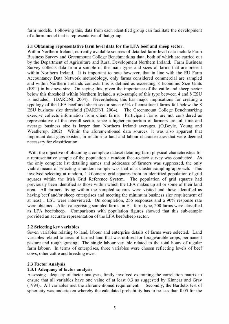
groupings of farms exist and further aggregation is unjustified as suggested groups have distinct differences. 2.5 Cluster Validation As a means of assisting assessment of cluster validity, several approaches where adopted. Firstly, although final results were obtained from outlined clustering technique, comparisons were made previously against results from alternative clustering strategies. Although most alternate clustering techniques suggested different solutions a few did return results that were almost identical, therefore providing some credence to results. Secondly, the randomly splitting sample approach as outlined by Everitt et al (2001) was conducted. Results showed consistency whereby analyses were conducted on each sub-sample of the split sample. Within step two as suggested by Everritt et al (2001), cluster centroids of the first sub sample were used within analyses for the second sub-sample. In this instance the results were again consistent, with exception of aggregating sub-sample farms that were members of clusters one and four in the original solution. Finally, the approach adopted by Kobrich et al (2003) was conducted, whereby resulting cluster details were compared against perceived sector structure. At face value, cluster details illustrated that within each cluster, farms are relatively homogeneous, given compactness of cluster variable values measured via variance. Further to this, it is felt that the individual clusters reflected accurately distinctly different farming systems that exist within studied sector, whereby key features of business scale, land quality and enterprise mix are accountable. 3 Results As a means of describing details of the final cluster solution, both the mean and standard deviation of clustering variables values for each individual cluster are displayed within table 1. Following this a description of each of the resulting clusters is made and their defining characteristics are highlighted. Cluster one named ‘Minute Beef Farms’ consists of relatively miniature farm businesses with average farm size of 5.6 ESU, but they do constitute 27.9% of the sample. Examination of cluster membership shows that 64% of farms have beef cows with herds between two and eighteen cows, 89% of farms have other cattle with herds between two and thirty-one head and 25% of farms have breeding ewes with flocks between six and one hundred and twenty-five ewes. Cluster two named ‘Micro Beef Farms’ consists of relatively very small businesses averaging 12.9 ESU, but again representing an important proportion of the sample (25.9%). Within this cluster, 83% of farms have beef cows with herds between ten and thirty cows. Only 15.7% of farms have breeding ewes with flocks between five and eighty ewes. All farms have other beef cattle with herds between eleven and sixty-nine head. In summary, this cluster contains farms with a very small but quite good quality land area, focusing on cattle production. In comparison to cluster 1 much larger mean values for land, labour and enterprise variables exist. Table 1: Characteristics of the identified homogeneous groups within the sample of LFA
Beef and Sheep Farms.
Cluster one
Cluster two
Cluster three
Cluster four
Cluster five
Cluster six
Cluster seven
Cluster eight
Cluster nine
Cluster ten
9
Cluster size (Farms)
56 51 20 44 2 5 13 2 2 5
Silage/crops area (hectares) 1
3.25 (2.18)
8.79 (2.84)
6.62 (4.13)
15 (5.7)
65.16 (17.74)
39.98 (18.04)
22.17 (9.09)
16.19 (11.45)
34.4 (8.58)
11.41 (4.96)
Pasture land (hectares) 1
7.29 (3.87)
13.29 (5.76)
15.88 (9.35)
24.58 (12.44)
117.77 (41.78)
67.71 (11.88)
47.55 (16.42)
72.96 (63.12)
84.18 (16.03)
28.37 (16.65)
Rough grazing (hectares) 1
3.24 (4.89)
4.49 (6.88)
21.25 (19.90)
13.35 (21.59)
50.59 (14.31)
17.4 (9.66)
12.94 (16.4)
380.21 (232.1)
176.85 (55.52)
109.07 (94.91)
Total Regular Labour (hrs) 1
26.7 (14.27)
43.05 (17.3)
46 (20.57)
69.42 (30.33)
113 (15.56)
122.6 (21.01)
91.87 (28.1)
115 (35.36)
155 (7.07)
68.4 (26.17)
No. Beef cows1
5.98 (5.5)
15.1 (8.43)
9.35 (9.28)
27.32 (12.84)
158 (31)
84.2 (30.71)
48.85 (20.35)
20.5 (0.71)
82.5 (38.89)
23.8 (22.53)
No. Other Cattle1
11.41 (7.87)
30.22 (12.78)
15.75 (13.15)
52 (19.1)
297.5 (137.9)
142 (45.21)
103.77 (54.17)
18 (2.82)
227 (21.21)
29.4 (26.97)
No. Breeding ewes1
12.45 (26.79)
6.76 (19.11)
111.85 (57.83)
31.4 (48.42)
0 19 (27.48)
70 (102.3)
1050 (212.1)
511 (182.4)
346 (122.9)
1. Standard deviations displayed in brackets
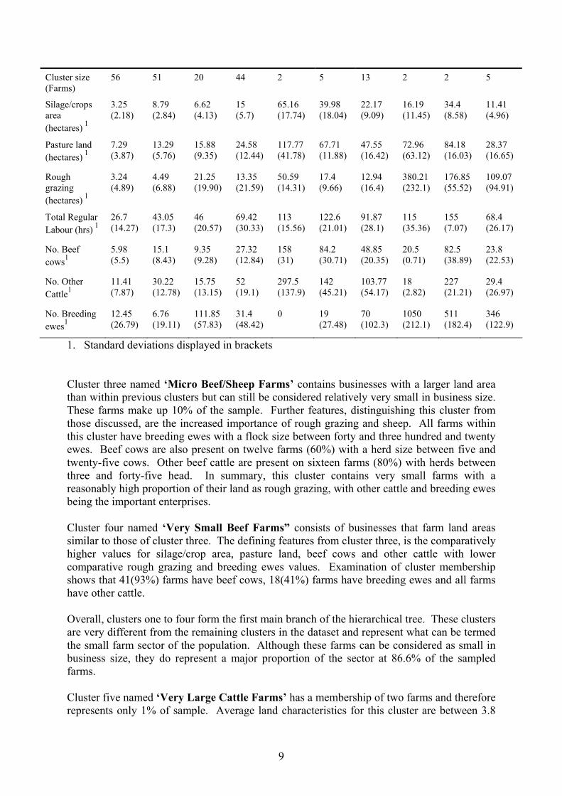
Cluster three named ‘Micro Beef/Sheep Farms’ contains businesses with a larger land area than within previous clusters but can still be considered relatively very small in business size. These farms make up 10% of the sample. Further features, distinguishing this cluster from those discussed, are the increased importance of rough grazing and sheep. All farms within this cluster have breeding ewes with a flock size between forty and three hundred and twenty ewes. Beef cows are also present on twelve farms (60%) with a herd size between five and twenty-five cows. Other beef cattle are present on sixteen farms (80%) with herds between three and forty-five head. In summary, this cluster contains very small farms with a reasonably high proportion of their land as rough grazing, with other cattle and breeding ewes being the important enterprises. Cluster four named ‘Very Small Beef Farms” consists of businesses that farm land areas similar to those of cluster three. The defining features from cluster three, is the comparatively higher values for silage/crop area, pasture land, beef cows and other cattle with lower comparative rough grazing and breeding ewes values. Examination of cluster membership shows that 41(93%) farms have beef cows, 18(41%) farms have breeding ewes and all farms have other cattle. Overall, clusters one to four form the first main branch of the hierarchical tree. These clusters are very different from the remaining clusters in the dataset and represent what can be termed the small farm sector of the population. Although these farms can be considered as small in business size, they do represent a major proportion of the sector at 86.6% of the sampled farms. Cluster five named ‘Very Large Cattle Farms’ has a membership of two farms and therefore represents only 1% of sample. Average land characteristics for this cluster are between 3.8
10
and 4.4 times the values within cluster four. In addition to this, the number of beef cows and other cattle are around 5.7 to 5.8 times the average values for cluster four. Beef cows and other cattle are the only enterprises present within this cluster. Cluster six named ‘Large Cattle Farms’ also consists of predominant cattle farms, operating on a smaller scale than those within cluster five in terms of land and enterprise characteristics. Cluster membership consists of five farms therefore representing 2.5% of the sample. In relation to enterprise mix, all farms have beef cows with herds between forty and one hundred and fifteen head. All farms also have other cattle with between eighty-six and two hundred head. Only two farms have breeding ewe enterprises, with flock sizes of thirty-five and sixty ewes respectively. In contrast, similar levels of labour input exist within clusters five and six. Overall it seems that cluster six is a scaled down version of cluster five but with similar levels of total labour input. Cluster seven named ‘Medium Beef farms’ contains thirteen farms, thus representing 6.5% of population. Cluster land details can be considered scaled down versions of cluster six as similar proportions of land farmed as silage/crops, pasture and rough grazing exist. This cluster is also relatively more focused on other cattle and sheep and less focused on beef cows than cluster six. Within this cluster twelve farms (92%) have beef cows with herds between thirty and eighty-four cows, all farms have other cattle with herds between forty-four and two hundred and thirty-five head and six farms (46%) have breeding ewes with flocks between twenty and two-hundred and eighty-five head. Overall, clusters five to seven represent different scales of production for predominate beef farms that are relatively large businesses compared to farms within clusters one to four. Clusters five to seven form the second main branch of the hierarchical tree. Cluster eight named ‘Very Large Cattle/Sheep Farms’ contains two farms, therefore representing 1% of population. Both these farms have beef cows, other cattle and sheep enterprises. Key differences exist between farms within this cluster and previously discussed clusters. Firstly, in terms of land utilisation, only a minor percentage is used for silage/crops (3.5%) in comparison to previous clusters, where a range in percentages between 15% and 33% exists. A second distinguishing feature is the large percentage (81%) of land that is rough grazing. Thirdly, the enterprise mix is predominately sheep with cattle numbers comparatively minor. Cluster nine named ‘Large Cattle/Sheep Farms’ also contains two farms and accounts for 1% of population. Compared to previous cluster, important similarities and differences exist. Firstly, in terms of land, cluster eight farms a larger area, has a lower proportion utilised for forage/arable production, has a higher proportion for rough grazing, but similar levels of pasture land exist. Secondly, cluster nine has a relatively higher predominance of suckler cows and other cattle, but a lower predominance of breeding ewes. Cluster ten named ‘Medium Cattle/Sheep Farms’ contains five farms therefore representing 2.5% of population. This cluster can be considered as having relative characteristics that are a hybrid of clusters eight and nine. In terms of land utilisation, 7.2% is used for forage/arable production, a value between that of clusters eight and nine. 17.9% of land farmed is used for pasture, a value similar to that of cluster eight. Rough grazing account for 69% of the land, a percentage almost exactly between that within cluster eight and nine. In terms of enterprise mix, 4 farms (80%) have beef cows, 4 farms (80%) have other cattle and all farms have
11
breeding ewes. Beef cows and other cattle levels are very similar to those of cluster eight whereas breeding ewe numbers are close to that of cluster nine. Overall, the previous three clusters contain businesses that farm large areas, of which a relatively large proportion is rough grazing. These farms constitute the third and final branch of the hierarchical tree. Within these results, a key finding is importance of the small farm component within studied sector, considered as consistent farms of clusters one to four. In total 171 farms are within these clusters, compared to only 29 farms within the large farm sector incorporated within clusters five to ten. Not only is this small farm sector important in terms of sectors businesses but also percentage of sectors beef cows (59.5%), other cattle (59.2%) and breeding ewes (44.3%). 4 Discussion and Conclusions The final factor analysis indicates that there are two underlying constructs that characterise the farming systems operated within the studied sector. A key feature of these constructs is the relationship between land quality and enterprise mix. Therefore, as we would expect, enterprise gross margins are not the sole consideration in selecting enterprise mix, as important land quality characteristics weigh heavily in determining the farming system operated. Further, although important to both factors, labour loaded more highly upon the beef production factor, indicating that this factor accounts for a higher amount of labour variance within the dataset than that caused by sheep production. From this we can deduce that similar proportional changes within the beef element of the studied sector will weigh more highly than changes within the sheep element upon the labour profile of these farms. In examining cluster analysis results, it is clear that there is a great deal of variability within the LFA beef and sheep sector of Northern Ireland. However, this variability is skewed towards a significant small farm element within the sector, represented by clusters one to four. The farms within these clusters not only account for a large percentage (85.5%) of this sectors businesses, but also for a high proportion of its beef herd and sheep flock. Therefore it is important to include these small farms within any analyses aimed to identify appropriate agricultural/environmental policy or farm management plans for this sector of the industry. Only focusing on what can be termed commercial businesses within this sector would be misleading. Overall, the multivariate techniques applied in this instance were successful in identifying, firstly, the constructs that characterise these farms, and secondly, the relatively homogeneous farm groups present. 5Acknowledgements The Livestock and Meat Commission for Northern Ireland and the Vaughan Trust jointly funded the work on which this article is based. 6 References Aldenderfer, M.S. and Blashfield, R.K. 1984. “Cluster Analysis”. Sage, CA, 88 Pages. Bernhardt, K.J., Allen, J.C. and Helmers, G.A. 1996. Using cluster analysis to classify farms for conventional/alternative systems research. Review of Agricultural Economics 18(4): 599-611.

12
Byerlee, D., Collinson, M., Perrin, R., Winkelmann, D., Biggs, S., Moscardi, E., Martinez, J.C., Harrington, L. and Benjamin, A. 1980. Planning Technologies Appropriate to Farmers – Concepts and Procedures, CIMMYT, Mexico, Child, D. 1990. “The essentials of Factor Analysis”. (2nd edition). Cassell Educational Limited, London, 120 Pages. Comrey, A.L and Lee, H.B. 1992. “A First Course in Factor Analysis”. (2nd Edition). Lawrence Erlbaum Associates Publishers, New Jersey, 430 Pages. DARDNI. 2004. “Farm Incomes in Northern Ireland 2002/03”. HMSO, Norwich, 89 Pages. Evans, R.D., Dillion, P., Shalloo, L., Wallace, M. and Garrick, D.J. 2004. An economic comparison of dual-purpose and Holstein-Friesian cow breeds in a seasonal grass-based system under different milk production scenarios. Irish Journal of Agricultural and Food Research, 43: 1-16. Everitt, B.S and Dunn, G. 1991. “Applied multivariate data analysis”. Edward Arnold, London, 304 Pages. Everitt, B.S., Landau, S. and Leese, M. 2001. “Cluster Analysis”. (4th Edition). Arnold, London, 237 Pages Field, A. 2000. “Discovering statistics using SPSS for windows”. Sage Publications, London, 496 Pages Hair, J.F. Jr., Anderson, R.E., Tatham, R.L. and Black, W.C 1998. “Multivariate Data Analysis”. (5th Edition) Prentice Hall, New Jersey, 730 Pages. Hardiman, R.T., Lacey, R. and Yi, Y.M. 1990. Use of cluster analysis for identification and classification of farming systems in Qingyang County, Central North China. Agricultural Systems 33: 115-125. Hennessy, T. 2000. Dairy farming in a booming economy and Agenda 2000. Journal of Farm Management 10(11): 653-664. Ketchen, D.J.Jr. and Shrook, C.L. 1996. The application of cluster analysis in strategic management research: An analysis and critique. Strategic Management Journal 17(6): 441-458. Kinnear, P.R and Gray, C.D. 1994. “SPSS for windows made simple”. Lawrence Relbaum, Hove, 275 Pages. Kline, P. 1994. “An Easy Guide to Factor Analysis”. Routledge, London, 194 Pages Kobrich, C., Rehman, T. and Khan, M. 2003. Typification of farming systems for constructing representative farm models: two illustrations of the application of multi-variate analyses in Chile and Pakistan. Agricultural Systems 76: 141-157.
13
Leeson, J.Y., Sheard, J.W. and Thomas, A.G. 1999. Multivariate classification of farming systems for use in integrated pest management studies. Canadian Journal of Plant Science 79: 647-654. Milan, M.J., Arnalte, E. and Caja, G. 2003. Economic profitability and typology of Ripollesa breed sheep farms in Spain. Small Ruminant Research 49: 97-105. Milligan, G.W. and Cooper, M.C. 1985. An Examination of Procedures for Determining The Number of Clusters In a Data Set. Psychometrika 50(2): 159-179. Monjena, R.1977. Hierarchical grouping methods and stopping rules: An evaluation. The Computer Journal 20(4): 359-363. Norusis, M. 2004. “SPSS 12.0 Statistical Procedures Companion”. Prentice Hall, New Jersey, 601 Pages. O’Boyle, J., Young, N. and Weatherup, N. 2002. “Suckler cows, beef and sheep benchmarking”. Greenmount College, Antrim, 20 Pages.