Equation Chapter 1 Section 1
Trabajo Fin de Máster
Máster Universitario en Electrónica, Tratamiento
de Señal y
Comunicaciones
Electrónica, Tratamiento de la Señal y
Comunicaciones
Construcción de una cámara semianecoica para test de
componentes de automoción
Autora: Carmen Ramírez Perdigón
Tutor: Luis Javier Reina Tosina
Dpto. Teoría de la Señal y Comunicaciones
Escuela Técnica Superior de Ingeniería
Universidad de Sevilla
Sevilla, 2018
Trabajo Fin de Máster
Máster Universitario en Electrónica, Tratamiento
de Señal y
Comunicaciones
Electrónica, Tratamiento de la Señal y
Comunicaciones
Construcción de una cámara semianecoica para test de
componentes de automoción
Autora: Carmen Ramírez Perdigón
Tutor: Luis Javier Reina Tosina


Trabajo Fin de Máster
Máster Universitario en Electrónica, Tratamiento de Señal y Comunicaciones
Construcción de una cámara semianecoica para test
de componentes de automoción
Autora:
Carmen Ramírez Perdigón
Tutor:
Luis Javier Reina Tosina
Profesor Titular de Universidad
Dpto. de Teoría de la Señal y Comunicaciones
Escuela Técnica Superior de Ingeniería
Universidad de Sevilla
Sevilla, 2018


Trabajo Fin de Máster: Construcción de una cámara semianecoica para test de componentes de
automoción
Autora: Carmen Ramírez Perdigón
Tutor: Luis Javier Reina Tosina
El tribunal nombrado para juzgar el Proyecto arriba indicado, compuesto por los siguientes miembros:
Presidente:
Vocales:
Secretario:
Acuerdan otorgarle la calificación de:
Sevilla, 2018

El Secretario del Tribunal

A mi familia
A mis maestros


Agradecimientos
Este trabajo final de máster no se podría haber llevado a cabo sin el apoyo de esas personas que me han
enseñado durante mi etapa académica, mis profesores. Especialmente agradezco al tutor de este trabajo,
Javier Reina, quien a pesar de la distancia a la que se realizó este TFM, fue paciente con mis errores y me
ayudó a la realización de éste.
A mis familiares, quienes me apoyaron en momentos de flaqueza y siempre creyeron en mi potencial. A
mi pareja por su paciencia y darme su opinión cuando dudaba.
A mis jefes y compañeros, ellos me han enseñado todo lo que sé respecto al sector de la compatibilidad
electromagnética en el sector de la automoción. Especialmente quiero agradecer a Jose María Laborda,
quien me dio la oportunidad de participar en este proyecto y quien me ha enseñado tanto.
Carmen Ramírez Perdigón
Barcelona, 2018


Resumen
En este trabajo fin de máster se presenta una solución al problema de la construcción de una cámara
semianecoica para componentes de automoción, tratando de plasmar los requerimientos necesarios
para construirla, un método para validarla y finalmente su puesta en marcha. Es un proyecto de
ingeniería que se llevó a cabo entre 2017 y 2018 en la empresa Applus Laboratories, situada en
Bellaterra (Barcelona).


Abstract
In this proyect, a solution is presented when building a semi-anechoic chamber for automotive
components, trying to show the necessary requirements to build it, a method to validate it and finally its
start-up. It was an engineering project that was carried out between 2017 and 2018 in the company Applus
Laboratories, located in Bellaterra (Barcelona).


Índice
Agradecimientos 9
Resumen 11
Abstract 13
Índice 15
Índice de Figuras 17
Acrónimos 19
1 Introducción 1 1.1 MOTIVACIÓN 4 1.2 OBJETIVOS 4 1.3 ESTRUCTURA 5 1.4 ANTECEDENTES Y ESTADO DEL ARTE 5
1.4.1 Honeycombs 6 1.4.2 Absorción de las ondas reflejadas dentro de cámara 6
2 Material y método 9 2.1 MATERIAL Y METODO 9 2.2 NORMATIVA APLICABLE A LA CONSTRUCCION DE UNA SAC 9 2.3 NORMATIVA DE VALIDACIÓN 11
2.3.1 Anexo J. 11 2.3.2 Medición de intensidad de campo 13
2.4 ACCESORIOS Y EQUIPAMIENTO 15 2.4.1 Cableado para RF 15 2.4.2 Comunicaciones usadas en una cámara semianecoica 16 2.4.3 Fibras ópticas 17 2.4.4 Transceivers 17 2.4.5 Monitorización por video 18 2.4.6 Transductores 19 2.4.7 Receptores de emisión 20 2.4.8 Generadores de señal de RF 21 2.4.9 Amplificadores de señal 22 2.4.10 Acoplador direccional 23 2.4.11 Medidores de potencia y sensores de potencia 24 2.4.12 Software 25 2.4.13 LISN (Line Impedance Stabilization Network) 25
3 RESULTADOS 27 3.1 ELECCIÓN DE LA CÁMARA 27 3.2 RESTRICCIONES RESPECTO AL ESPACIO DE CONSTRUCCIÓN 27 3.3 ADAPTACIÓN PARA SAC 4 DE LOS ELEMENTOS DE LA CÁMARA ANTIGUA 29
3.3.1 Paneles metálicos para el blindaje 29 3.3.2 Puerta 33 3.3.3 Climatización de la sala 34 3.3.4 Filtros de tensión 34 3.3.5 Caminos de RF (trampillas y conectores) 37

3.3.6 Absorbentes piramidales y baldosas de ferrita 38 3.3.7 Plano de masa de referencia 39
3.4 OBRA 40 3.4.1 Mejora de la red de alimentación y aislamiento eléctrico 43
3.5 EJECUCIÓN DE LA VALIDACIÓN Y RESULTADOS 44 3.5.1 Resultado de las mediciones 44
4 Conclusiones 48 4.1 LINEAS FUTURAS 48
Anexos 48
Referencias ¡Error! Marcador no definido.

ÍNDICE DE FIGURAS
Figura 1:Esquema de test de EMI o EMS 2 Figura 2: Cámara de Faraday 2 Figura 3: Interior de una cámara semi-anecoica en Applus 3 Figura 4: Cámara completamente anecoica. 3 Figura 5: Distintos tipos de absorbentes para cámaras semianecoicas 7 Figura 6: Absorbentes de tipo cuña. 7 Figura 7: Otros tipos de absorbentes. 8 Figura 8: Efecto onda absorbida. 10 Figura 9: Influencia de la conexión del plano de masa, los absorbentes y el plano de masa (Anexo J de la CISPR25). 11 Figura 10: Equipo emisor de señal. 12 Figura 11: Plano para el montaje del equipo emisor. 12 Figura 12: Plano de los conectores del equipo emisor. 12 Figura 13: Esquema del test de validación con antena monopolo. 14 Figura 1: Estructura de comunicaciones LIN en una SAC. 17 Figura 15: Modulos transceiver de Messtechnik. 18 Figura 16: Cámara portátil y cámara fija de Messtechnik. 19 Figura 17: Distintos módulos controladores de cámara. 19 Figura 18: Diferentes tipos de transductores. 20 Figura 19: Estructura de un receptor de señal. 21 Figura 20: Receptor ESW 8 de Rohde & Schwarz. 21 Figura 21: Señales generadas más usuales. 22 Figura 22: Generador de Rohde & Schwarz. 22 Figura 23: Zona lineal de trabajo del amplificador de señal. 23 Figura 24: Acoplador direccional de 40 dB. 23 Figura 25: Esquema de funcionamiento del acoplador direccional. 24 Figura 26: Sensor de potencia de R&S Z-91. 25 Figura 27: Vista de las conexiones de un Hardware setup en el EMC32. 25 Figura 28: Esquema del interior de una LISN. 26 Figura 29: LISN de Schwarbeck Mess-Elektronik. 26 Figura 30: Distribución del nuevo laboratorio para autocomponentes. 28 Figura 31: Espacio para la construcción de SAC4 28 Figura 32: Vista de la planta de la SAC original (techo). 29 Figura 33: Vista de la planta de la SAC original (suelo) 30 Figura 34: Vista trasera de la SAC original. 30 Figura 35: Vista frontal de la SAC original. 30 Figura 36: Vistas laterales de la SAC original. 31 Figura 37: Vista de la planta de SAC4 (techo) 31 Figura 38: Vista de la planta de SAC 4 (suelo) 32 Figura 39: Vistas laterales de SAC 4. 32 Figura 40: Paneles de la SAC original que no se reutilizaron. 33 Figura 41: Puerta SAC original / SAC 4. 34 Figura 42: Setup típico para emisiones radiadas en bajas frecuencias (antena monopolo) 35 Figura 43: Filtros de 32 A. 36 Figura 44: Paneles con filtros nuevos. 36 Figura 45: Plano de los caminos de RF. 37 Figura 46: Localización de los caminos de RF 38 Figura 47: Vista superior la cámara con absorbentes reciclados y nuevos. 39

Figura 48: Vista superior de la cámara incluyendo la mesa. 40 Figura 49: Vista lateral y vista frontal de la posición de la mesa dentro de la cámara. 40 Figura 50: Nivelado del emplazamiento de SAC 4. 41 Figura 51: Montaje de la estructura blindada. 41 Figura 52: Recubrimiento de baldosas de ferrita durante la obra. 42 Figura 53: Absorbentes en el techo de SAC 4. 43 Figura 54: Plano de masa de referencia atornillado al blindaje de SAC 4. 43 Figura 55: Zonas de red de alimentación. 44 Figura 56: Desviación con la antena ROD (150 kHz- 30 MHz) (escala lineal). 45 Figura 57: Desviación con la antena bicónica (30 MHz- 200 MHz) (escala lineal). 45 Figura 58: Desviación con la antena logo periódica (200 MHz- 1 GHz) (escala lineal). 46 Figura 59: Resultado de la desviación total (escala logarítmica). 46 Figura 60: Cableado de RF para equipar SAC 4 ¡Error! Marcador no definido.

Acrónimos
EUT
EMC
Equipment under test (equipo bajo test)
Electromagnetic compatibility (compatibilidad electromagnética)
EMI Referente a los test de emisiones
EMS
SAC
FAC
Referente a los test de inmunidad
Semi-anechoic chamber (cámara semi-anecoica)
Faraday chamber (jaula de Faraday)
SR
ESD
AP1
AP2
RF
Shielded room (sala apantallada)
Electrostatic discharge (descarga electrostática)
Panel de conectores 1
Panel de conectores 2
Radio frecuencia


1 INTRODUCCIÓN
Desde los albores de las comunicaciones por medio de ondas electromagnéticas, se tuvo consciencia de la
necesidad de evitar las interferencias entre distintas emisiones y de una sana convivencia entre los toscos
receptores de la época. De los primeros aparatos de radio que carecían de selectividad y se podían escuchar
varias emisoras al mismo tiempo se pasó a los receptores superheterodinos, que eran modelos más avanzados
técnicamente, los cuales garantizaban estabilidad de funcionamiento y, sobre todo, selectividad de la emisora
escuchada, con una mejor protección frente a interferencias.
Con el tiempo y el avance de la tecnología se fue abriendo paso a una nueva disciplina científico-tecnológica,
la compatibilidad electromagnética (también conocida por sus siglas CEM o EMC) que se define como la
rama de la tecnología electrónica y de las telecomunicaciones que estudia los mecanismos para eliminar,
disminuir y prevenir los efectos de acoplamiento entre un equipo eléctrico o electrónico y su entorno
electromagnético, intentando incorporar este conocimiento desde las primeras etapas de diseño de los
dispositivos y sistemas.
Actualmente, la compatibilidad electromagnética se regula mediante normas y estándares con la finalidad de
asegurar la confiabilidad y seguridad de los equipos y sistemas. Para cumplir con estos estándares se debe
realizar la comprobación del funcionamiento electromagnético del equipo mediante las pruebas establecidas
por el estándar regulador.
Posiblemente los pioneros de estos estudios hayan sido la industria militar y la aviación. La posibilidad de
un fallo, debido a una deficiente compatibilidad electromagnética en ambas actividades, podría tener
consecuencias catastróficas. En la electrónica de consumo y en automoción, los estándares que rigen el
comportamiento de los productos electrónicos frente a la compatibilidad electromagnética se han ido
ampliando y cobrando importancia con el paso de los años.
Un ejemplo de la importancia de la compatibilidad electromagnética en el sector de automoción es el
siguiente. Imaginemos un vehículo que circula por la noche (éste será la víctima) y que, debido a una
interferencia electromagnética generada por la señal radar (fuente de interferencia) de un aeropuerto cercano,
acciona por error las luces de freno. El conductor de un vehículo que circule por detrás del anterior, al
observar las luces de freno, para evitar una colisión, también frenará, posiblemente sin que le dé tiempo de
ver si circulan coches por detrás. Esta situación puede causar un accidente y es perfectamente evitable. En
España se vendieron, solo durante 2017, 1.462.230 vehículos nuevos (1) y todos están expuestos a campos
electromagnéticos que podrían causar situaciones similares o peores que la anterior. La importancia de la
compatibilidad electromagnética, en un sector que es además cada vez más electrónico, es innegable.
Como ya hemos dicho, la regulación de EMC se realiza mediante tests prestablecidos. Se distinguen dos
grandes grupos de pruebas según la funcionalidad: de inmunidad, normalmente nombrados con las siglas
EMS, y de emisiones, normalmente conocidos
por las siglas EMI. En los primeros se trata de comprobar la robustez que tiene el equipo ante posibles
interferencias que provengan de su entorno. Para los test de emisiones sería el caso contrario, la norma
establece unos niveles máximos de emisión que no se deben sobrepasar para que el equipo bajo prueba no
interfiera en su entorno (véase la figura 1).

Figura 1:Esquema de test de EMI o EMS.
También pueden considerarse dos categorías según el tipo de propagación electromagnética: propagación
conducida o radiada. Un test de inmunidad conducida, por ejemplo, consiste en inyectar una corriente
mediante una pinza (transductor) al cableado de un equipo y comprobar cómo reacciona el equipo bajo
prueba. Por su parte, un test de inmunidad radiada consiste en irradiar el equipo bajo prueba con un campo
electromagnético mediante una antena.
Las pruebas de conformidad requieren un entorno caracterizado y seguro donde puedan realizarse. Para ello
existen diferentes alternativas, dependiendo del grado de apantallamiento que sea preciso considerar:
Cámara o jaula de Faraday, también conocida como cámara o sala apantallada o por sus siglas en
inglés, FAC y SR (figura 2). Este tipo de cámaras proporcionan aislamiento electromagnético, es
decir, las señales de RF que se encuentran en su interior no pueden salir y viceversa. Está compuesta
básicamente por una estructura metálica con una puerta que garantiza un cierre con buen contacto
metálico.
En su interior, las ondas electromagnéticas pueden estar sometidas a reflexiones que son difíciles de
controlar, por lo que este entorno no se considera apropiado para realizar tests de emisiones o
inmunidad radiadas. Sin embargo, estos lugares son útiles para realizar tests conducidos, donde las
componentes radiadas y reflejadas apenas tienen efecto.
Figura 2: Cámara de Faraday
Cámaras semi-anecoicas (figura 3), normalmente conocidas por sus siglas en inglés, SAC (semi-
anechoic chamber). Estas salas proporcionan no solo aislamiento electromagnético, sino que además
simulan condiciones de espacio libre de influencias electromagnéticas. Se trata de las cámaras
comúnmente usadas en la industria de automoción para tests de emisiones o inmunidad radiadas, ya que
son capaces de absorber las señales reflejadas en paredes y techo, aunque no en el suelo. El suelo será

un plano de masa que simulará las condiciones electromagnéticas reales, donde un vehículo circula
sobre un plano de masa que será el suelo.
A lo largo de este trabajo se describirá este tipo de cámaras de forma más extensa, indicando cuáles son
las características físicas de la cámara y de los materiales utilizados y por qué se usan de una manera y
no de otra. Se abordarán los problemas que plantea el diseño, implementación y puesta en marcha de
una SAC para componentes de automoción y cómo se pueden solucionar, llegando finalmente a la
validación, lo que indicará que la cámara cumple los requisitos establecidos por los clientes y las
entidades reguladoras.
Figura 3: Interior de una cámara semi-anecoica en Applus.
Cámaras completamente anecoicas, normalmente conocidas como FAC (del inglés, Full Anechoic
Chamber). Estas salas (figura 4), a diferencia de las anteriores, proporcionan un espacio completamente
libre de reflexiones, incluidas las del suelo. Este entorno resulta útil para ciertos test de compatibilidad
electromagnética en determinadas aplicaciones industriales y especialmente en el ámbito de la
aeronáutica.
Figura 4: Cámara completamente anecoica.

1.1 MOTIVACIÓN
En el contexto de la automoción, la obligación de testear la compatibilidad electromagnética de cada equipo
que se instale en un vehículo a motor, supone una gran cantidad de trabajo y también de tiempo, debido al
enorme número de componentes. Sin embargo, no existen, al menos en España, suficientes laboratorios
acreditados que proporcionen estos servicios a la industria.
Las principales empresas que realizan esta actividad en España se encuentran en Cataluña, ya que es el
principal foco de la industria de automoción en nuestro país. Estas son Applus, donde se ha desarrollado este
trabajo, e Idiada. Fuera de nuestro país encontramos importantes laboratorios de EMC para automoción,
como 3Ctest en Reino Unido (recientemente adquirido por Applus).
Otra posibilidad para las empresas y fabricantes de estos productos es que realicen sus propias validaciones
si disponen de los medios necesarios y consiguen las acreditaciones. Este es el caso de Lear, en Tarragona.
Sin embargo, no solo es tremendamente costoso tener un laboratorio con todo el equipamiento necesario para
realizar validaciones, sino que también es complicado, una vez montado el laboratorio, cumplir con todos
los parámetros necesarios para que a ese laboratorio se le otorguen las acreditaciones. Por ello, la mayoría de
las empresas optan por subcontratar estos servicios.
El problema que encuentran cuando solicitan un test de EMC es, en muchas ocasiones, el tiempo de espera.
Aunque este tiempo depende del tipo de test, de lo complicado que pueda ser el montaje del setup o de si se
trata o no una validación completa, es habitual que los tiempos oscilen entre 1 y 11 semanas. Esta amplitud
lleva en ocasiones a tener que externalizar el test, si estos son urgentes, a otros países, en ocasiones mucho
más costosos que en España.
El hecho de disponer de una nueva cámara SAC supondría reducir estos tiempos de espera y, obviamente,
abarcar muchos más trabajos que poder facturar, razones que justifican la necesidad del presente Trabajo Fin
de Máster.
Es preciso referirse al reto que supone, tanto empresarial como personal, la realización de este Trabajo Fin
de Máster. Empresarial, debido al coste y a la inversión de recursos, y personal, ya que plantea una temática
que requiere una alta cualificación científico-tecnológica y no existen directrices armonizadas a la hora de
abordar el diseño de cámaras semianecoicas para automoción.
Cuando entré a formar parte del proyecto ya había terminado la fase de planteamiento y aceptación de la
obra, pero aún quedaba realizar la obra, la validación y la compra de todos los equipos. Durante estos meses
he combinado mi trabajo como ingeniera de test en una cámara de Faraday con el proyecto de la nueva
cámara. Desde Applus realizamos el estudio de los equipos necesarios, los cálculos para las dimensiones del
cableado y fibras, se realizó la supervisión de la construcción y la validación posterior y en todo momento
Albatross, empresa encargada de la obra, trabajó bajo las directrices impuestas por Applus para la mejora de
la cámara.
1.2 OBJETIVOS
El objetivo principal de este trabajo es plasmar de forma clara los procesos necesarios para diseñar y
desplegar una cámara semianecoica para componentes de automoción (autocomponentes) completamente
operativa, llamada SAC 4, proporcionando una metodología sistemática que ayude a la armonización de los
procesos.
Para alcanzar este objetivo principal será necesario cumplir los siguientes objetivos particulares:
Elegir la construcción que mejor se adapte a las necesidades de la empresa para la obtención de la
SAC.

Construcción de la SAC.
Validación de la SAC, donde se explicará el método elegido y se pondrá en práctica, obteniendo
finalmente unos resultados.
Dotar del equipamiento necesario a la SAC para que esté completamente operativa.
1.3 ESTRUCTURA
La estructura de este proyecto está redactada enmarcando primero el marco teórico en el que se encuentra
éste trabajo. Dónde primero se estudia la normativa aplicable a una cámara semianecoica del sector de la
automoción y se proponen dos métodos de validación.
Después, también en un marco teórico, se indican los equipos y accesorios necesarios para trabajar con ésta
cámara.
Una vez visto todo lo necesario para una nueva cámara semianecoica, lo siguiente es buscar, de entre las
distintas opciones, que cámara se adecua mas a las necesidades del laboratorio, optándose por comprar y
reciclar la cámara de otra empresa.
Debído a que la cámara original no se adecúa a los estándares de automoción es necesario hacer una
readaptación, aprovechando el mayor material posible, para crear la núeva cámara.
Con la estructura de SAC4 ya planteada se realiza la construcción y de ésta, la posterior validación.
Finalmente, se hace un análisis de las conclusiones obtenidas del Trabajo Fin de Máster y una propuesta de
líneas futuras.
1.4 ANTECEDENTES Y ESTADO DEL ARTE
No existen suficientes precedentes de estudios que se desarrollen la metodología seguida durante la
construcción de una cámara semianecoica. Sin embargo, sí que se pueden citar estudios de rendimiento de
estas cámaras, por ejemplo [2]. En este artículo se estudia la importancia del plano de masa y de su conexión
a la cámara y cómo conseguir un plano de masa con menor resonancia. Además, en nuestro país existen
publicación que los ingenieros de diseño toman como referencia para aprender a realizar diseños teniendo en
cuenta la compatibilidad electromagnética, una de estas publicaciones viene a cargo del ingeniero Joan Pere
Lopez Veragua., [3].
En Applus se realizó un proyecto similar un año antes de comenzar con el planteamiento de SAC 4, la
construcción de SAC 3, que además, se convirtió en la primera cámara semi-anecoica de estas características,
diseñada y planificada en España, ya que el proyecto se llevó a cabo íntegramente por Applus.
La construcción de SAC 3 tiene ciertas similitudes con la de SAC 4, ya que fue la readaptación de una cámara
que poseía Applus desde hacía 30 años, pero que estaba en desuso. La empresa vio la oportunidad de utilizar
los materiales y el espacio que poseían la antigua cámara, modificarla para que se adecuara a la normativa
actual, e intentar ponerla en marcha, todo esto por un coste mucho menor que el de adquirir una cámara
nueva.
Se tuvo que desmantelar completamente la cámara para comprobar el estado del blindaje, ya que con el paso
del tiempo había sufrido corrosión por humedad. El blindaje exterior se reparó y se mejoró, ya que existían
puntos de discontinuidad. Se incorporaron baldosas de ferritas a paredes y techo, ya que la antigua cámara
no las tenía y se incorporaron los absorbentes que se habían desmontado. La planificación y construcción de
SAC 3 se realizó entre 2016 y 2017, entrando en funcionamiento en mayo de 2017.
Durante la realización de la construcción de SAC 3 se llevó a cabo el estudio de la normativa, se comprendió

cómo realizar una construcción de este tipo, se estudiaron los costes asociados y obviamente se cometieron
errores. Todo este aprendizaje sirvió para adquirir experiencia que permitiera afrontar la realización de SAC
4.
Las construcciones se realizan basándose en el estándar regulador vigente, por ejemplo, en el caso de equipos
industriales el estándar CISPR16, entendiendo por industriales los equipos comercializados que no requieran
una seguridad especial como por ejemplo lavadoras, equipos de sonido, etc.
El último estándar regulador de automoción, la norma la CISPR 25 Ed.4 (15-05-2015), anexo 1 de esta
memoria, incluye por primera vez un apartado con métodos para validar el correcto comportamiento de las
cámaras, el Anexo J. Antes de la aparición de este anexo el estándar CISPR 25 se limitaba a ofrecer
indicaciones sobre la construcción, pero no solicitaba ningún tipo de medición que caracterizara la cámara.
Aunque el Anexo J no es de obligatorio cumplimiento es altamente recomendable tenerlo en cuenta para
realizar nuevas cámaras. Además, se prevee que para conseguir las futuras acreditaciones de los fabricantes
estos exijan la validación del Anexo J.
Para el cumplimiento de este anexo es necesario obtener un buen blindaje del exterior, siendo para ello muy
importantes los paneles de ventilación o honeycombs, y un buen nivel de absorción de las ondas reflejadas
en el interior de la cámara. Para esto último se utilizan absorbentes, este es el punto donde se ha visto el
mayor el desarrollo tecnológico respecto al desarrollo de cámaras semianecoicas, ya que las primeras
cámaras ni siquiera los incorporaban y su mejora es necesaria para bajar el nivel de ruido ambiental dentro
de una cámara.
1.4.1 Honeycombs
Dentro de la cámara es necesario incluir ventilación, para ello se utilizan los paneles denominados
honeycombs por la forma de su reja.
Estos paneles son tan importantes en el blindaje que normalmente determinan la frecuencia hasta la que la
cámara está blindada. Tienen dos factores fundamentales, el primero es la cantidad de aire que dejan pasar y
el segundo el blindaje que ofrecen. Estos factores suelen estar enfrentados, es decir, mientras mayor sea la
cantidad de aire que dejen pasar menor será el blindaje.
Una opción que nos proporcionan los fabricantes para obtener una mejor atenuación, sobre todo en
frecuencias altas donde el blindaje de los paneles deja de tener efectividad, es la de combinar paneles
cruzados, aunque esto disminuiría considerablemente el flujo de aire. Para mejorar el flujo de aire en el caso
que fuera necesario también es posible incorporar un ventilador al panel (fuera de la cámara).
1.4.2 Absorción de las ondas reflejadas dentro de cámara
Los absorbentes son los materiales encargados de absorber las ondas reflejadas en el interior de la cámara.
Existen dos grupos fundamentales de absorbentes, las ferritas y absorbentes de poliuretano.
Centrándonos primero en los absorbentes de poliuretano, a los que normalmente se les conoce como
absorbentes de RF, vemos que existe una gran tipología en el mercado, desde el material hasta la forma y
tamaño, los diferentes absorbentes se comportan de manera distinta.
El poliuretano es un material plástico poroso formado por una agregación de burbujas. Se forma básicamente
por la reacción química de dos compuestos, un poliol y un isocianato, aunque su formulación necesita y
admite múltiples variantes y aditivos. El poliuretano al ser dopado con carbón ofrece una buena absorción
de ondas electromagnéticas, dependiendo del porcentaje de carbón que tenga el poliuretano, absorberá más
o menos energía.
Las prestaciones de las pirámides absorbentes de poliuretano dependen de su altura, en la figura 5 vemos

distintos tipos de absorbentes según su altura. Cuanto mayor sea la altura de la pirámide (medida en
longitudes de onda), mayor será su absorción. Las pirámides absorbentes más comúnmente utilizadas son las
de 0.61 m, aunque su tamaño puede variar entre 0.1 m y 3m. La efectividad de las pirámides aumenta
conforme aumenta la frecuencia, ya que disminuye su longitud de onda. La desventaja de utilizar estas
pirámides es que, a frecuencias bajas, el tamaño de éstas para un correcto funcionamiento es demasiado
grande (más o menos 3 m) y esto supone una reducción importante del área útil de la cámara, salvo que se
usen en cámaras muy grandes.
Figura 5: Distintos tipos de absorbentes para cámaras semianecoicas
Otro factor que afecta a la absorción de la pirámide es el porcentaje de carbón, pues a medida que el
porcentaje de carbón aumenta, mejor es la absorción en altas frecuencias, pero peor para frecuencias bajas.
Otro factor a tener en cuenta es la forma, generalmente los absorbentes son cónicos o piramidales, pero a
veces se utilizan absorbentes de cuña, ejemplos de ello puede verse en la figura 6. Son utilizados
generalmente en cámaras anecoicas y semi-anecoicas estrechas. Este absorbente se diseñó principalmente
para dirigir la energía en un camino dado para que ésta pueda absorberse eficazmente por los otros materiales
absorbentes (pirámides).
Figura 6: Absorbentes de tipo cuña.
Otra forma, aunque menos habitual, es la pirámide girada, su punta esta girada 45º. La ventaja de utilizar
estos absorbentes es que utilizan menos material que la pirámide normal, y que sus puntas no se inclinan con
el paso de los años. Sin embargo, su absorción no es tan buena como la absorción de la pirámide normal.
Actualmente se estudian los denominados absorbentes de nueva generación, en los que cambia básicamente
su forma. En la figura 7 podemos ver nuevas formas diseñadas para absorbentes.

Figura 7: Otros tipos de absorbentes.
Por otra parte, otro tipo de absorbente, quizás el más conocido, es el absorbente magnético o ferrita. Las
baldosas de ferrita normalmente tienen buena absorción, (entre -10 dB y 30 dB) en el rango de frecuencias
de 30 MHz a 600 MHz, a partir 600 MHz el comportamiento empieza a empeorar. Hay que destacar que se
obtienen valores de absorción equivalentes a los que se obtendrían con pirámides de 3 m de longitud y una
carga de carbón alta, pero ocupando apenas un par de centímetros de la cámara.
Según las necesidades, es posible combinar ambos absorbentes, a esto se le denomina absorbente híbrido.
Teniendo en cuenta que los absorbentes de ferrita trabajan bien hasta más o menos 600 MHz y que los
absorbentes piramidales de tamaño medio (típicamente 60 cm) se puede cubrir la banda de frecuencias altas
(hasta 40 GHz).

2 MATERIAL Y MÉTODO
2.1 MATERIAL Y METODO
Se ha seguido la metodología de un proyecto de ingeniería llave en mano:
Identificación de requisitos mediante el estudio de la normativa del sector. Analizando el estándar
CISPR25, refente a lo ensayor de emisiones para componentes de automoción.
Especificación formal de requisitos, tanto para la construcción como para la validación de una
cámara semianecoica.
Especificación del equipamiento necesario para la puesta en marcha de la cámara.
Propuesta de solución tecnológica. Realización de planos para una cámara que se adaptase a los
requisitos ya estudiados.
Construcción y validación. Realización de la obra y posterior estudio del correcto apantallamiento
mediante la validación estudiada en el estándar CIPS25.
2.2 NORMATIVA APLICABLE A LA CONSTRUCCION DE UNA SAC
Antes de comenzar a plantear cualquier construcción fue necesario estudiar detenidamente los requisitos
exigidos por la normativa vigente, en este caso el estándar CISPR 25. Ésta es la norma fundamental que rige
los test de medición de emisiones para automoción y que será adaptada por cada fabricante (Mercedes Benz,
Renault-Nissan, Peugeot …) como base para establecer sus propias normas (igual o más exigentes que la
CISPR 25). Es decir, la cámara deberá cumplir, al menos, con las restricciones de la CISPR 25 y una vez
conseguido se deberá comprobar que también cumple con exigencias de cada fabricante para obtener la
acreditación para poder realizar tests de cada uno.
Lo primero que la CISPR 25 establece respecto a lo que debe cumplir una cámara para automoción (vehículo
y autocomponentes) son los niveles de ruido electromagnético ambiental que deben cumplirse en su interior.
Estos tienen que estar al menos 6 dB por debajo de los especificados por la norma. La norma también
proporciona unos límites de emisiones conducidas (punto 6.4.3 del anexo 1) y de emisiones radiadas (punto
6.5.4. del anexo 1) que los equipos bajo prueba deben superar.
Hay que tener en cuenta que dentro del blindaje habrá energía reflejada desde las superficies interiores. Este
tipo de energía no causa un gran problema a la hora de realizar mediciones de emisiones conducidas, con lo
que para este tipo de pruebas puede usarse, por ejemplo, una cámara de Faraday. Sin embargo, para
mediaciones de emisiones radiadas, la energía reflejada puede causar errores de hasta 20 dB. Por lo tanto, es
necesario aplicar algún material absorbente de RF a las paredes y al techo del blindaje. Como ya se vió, una
solución típica son los absorbentes de RF, normalmente ferritas para bajas frecuencias y conos para
frecuencias superiorres, estos son capaces de absorber la onda incidente (figura 8). No se debe colocar este
material en el suelo.
El material de absorción debe tener un rendimiento mayor o igual a 6 dB en el rango entre 70 MHz a 2500
MHz. Este rendimiento se refiere a la capacidad de disminuir el ruido ambiente que tiene el absorbente. El
estándar CISPR25 define, en el punto 4.1.4, que el ruido ambiente debe estar al menos 6 dB por debajo de
los límites de emisiones, si el ruido fuera superior es posible que camuflara la emisión que se desea medir.

Figura 8: Efecto onda absorbida.
Respecto al tamaño máximo o mínimo, la norma no indica nada, pero sí establece que el recinto deberá ser
de un tamaño lo suficientemente grande como para garantizar que tanto la antena como el equipo bajo prueba
(EUT, del inglés equipment under test) pueda colocarse a una distancia de un metro, al menos, de cualquier
punto de la sala, incluyendo el absorbente.
Para evitar posibles problemas, especialmente en tests de emisiones radiadas, dentro de la cámara no deberán
colocarse elementos innecesarios como armarios, sillas, etc. Cuando se realicen los tests, esta restricción
también incluye al personal que no participe activamente en su realización.
A diferencia de los tests para industria, todos los tests de componentes de automoción se realizan colocando
el EUT sobre un plano de masa de referencia. Este deberá ser una superficie realizada en cobre, latón, bronce
o acero galvánico, de al menos 0,5 mm de espesor. En nuestro caso, teniendo en cuenta que queremos poder
realizar tanto medidas de emisiones radiadas como para emisiones conducidas, el tamaño mínimo del plano
de tierra debe ser de 2,5 metros x 1 metro. El plano de masa tiene que estar elevado 0.9 ± 0.1 metros con
respecto al suelo de la cámara.
El plano de masa de referencia deberá estar unido por medio de unas tiras (straps) al blindaje de la cámara.
Las tiras estarán realizadas en uno de los materiales indicados anteriormente. La distancia entre las tiras no
puede ser mayor a 30 cm y se debe guardar una proporción entre la longitud y el ancho de las tiras de 7:1.
Para garantizar una conexión de baja impedancia a la sala blindada, es necesario un número suficiente de
straps.
Las resonancias del plano de tierra de referencia, la ubicación, el ancho y la longitud de los straps influyen
enormemente en los resultados de la medición. En la figura 9 se muestra la influencia del plano de masa.

Figura 9: Influencia de la conexión del plano de masa, los absorbentes y el plano de masa (Anexo J de la
CISPR25).
2.3 NORMATIVA DE VALIDACIÓN
Es necesario definir un método con el que comprobar el blindaje y, en general, el correcto funcionamiento
de una cámara semianecoica. El anexo J de la CISPR25 proporciona dos métodos que, aunque no de obligado
cumplimiento, son una buena práctica para validar una nueva SAC.
2.3.1 Anexo J.
La CISPR25 recomienda que se pruebe el rendimiento del blindaje de la cámara para configuraciones de test
de emisiones radiadas, es decir, donde el blindaje es más crítico. Con este procedimiento se evaluarán las
influencias de los absorbentes, el plano de tierra, la conexión al plano de tierra, etc.
La CISPR25 ofrece la opción o no de colocar baldosas de ferritas en el suelo. No será necesario poner suelo
de ferrita si la cámara sin ellas cumple con la validación expuesta en este anexo.
Los dos métodos descritos son los siguientes.
Método de medición de referencia. Este método utiliza un emplazamiento de referencia del cual ya
se conoce que cumple con los requisitos de la norma CISPR 16-1-4. Se tomarán medidas de una
señal emitida con una pequeña antena monopolo y luego se compararán las medidas del sitio de
referencia con las del sitio a validar. Las medidas deben quedar dentro de una tolerancia definida en
el anexo J de la CISPR25.
Método de antena modelada de cable largo. En este método se utiliza como antena transmisora un
cable de 50 cm. Se realizarán medidas a 30 MHz y superiores con test de emisiones radiadas. Las
medidas deben quedar dentro de una tolerancia determinada.
En este Proyecto nos centraremos en detallar únicamente el segundo método, ya que fue el elegido para
validar SAC 4. Todos los detalles de cómo realizar el primer método se encuentran bien definidos en el anexo
J.

Para el método elegido es necesario disponer del equipo que actuará a modo de antena emisora, en este caso
se trata de un alambre de 50 cm de longitud que se elevará 5 cm sobre el plano de masa y estará suspendido
entre dos placas metálicas cuadradas terminadas, por un lado, en una carga de 50 ohms y después en un
atenuador de 10 dB al que se le conectará el sistema de generación de señal (véanse las figuras 10, 11 y 12).
Figura 10: Equipo emisor de señal.
Figura 11: Plano para el montaje del equipo emisor.
Figura 12: Plano de los conectores del equipo emisor.
Los tipos de antena receptoras (según el rango de frecuencia que se vaya a medir) se describen en el punto
6.5 de la CISPR25 y serán una antena monopolo, una antena bicónica y una antena logoperiódica. Los
factores de antena (ganancia de cada antena) deben ser conocidos y considerados en los cálculos.
No es necesario que la potencia transmitida sea muy elevada, para evitar una sobrecarga del sistema de

emisión se inserta el atenuador de 10 dB y este factor se incluye en los cálculos de medida.
La configuración o esquema físico de todos los equipos que intervienen en la medición debe ser el mismo
que en un test de emisiones radiadas, las distancias, los caminos, etc.
El paso de frecuencias que se usará viene definido en el punto J.2.3.1.2 de la norma CISPR25.
2.3.2 Medición de intensidad de campo
El esquema de la configuración del test lo encontramos en la figura 13. La primera medida se debe hacer de
forma directa, con el cable que alimentará a la antena emisora (8) directamente conectado al cable de salida
de la antena receptora (7). El equipo que genere la señal debe estar configurado a 1 Vrms (120 dB(µV)). La
medida leída se representará como M0 en dB(µV).
Para la medida del coeficiente de radiación, es decir, que intensidad de campo eléctrico que recibe la antena,
se conecta el cable que transmite la señal de 1 Vrms (8) a la entrada del atenuador de 10 dB (3) y el cable del
receptor (7) se conecta a la antena receptora (6), según se muestra en la figura 39. Se configura de nuevo la
amplitud de la señal generada a 1 Vrms a la entrada del atenuador de 10dB. La lectura del receptor será
registrada como MA en dB(µV) ya que la antena habrá convertido la señal de campo eléctrico a tensión y
eso será lo que verá el receptor.

Figura 13: Esquema del test de validación con antena monopolo.
Es necesario tener las antenas que se usan caracterizadas con su factor de antena. Este factor se define como
la relación entre la intensidad es campo eléctrico y la tensión que se genera en los terminales de la antena.
A partir de los dos valores calculados y el factor de antena de la antena receptora (kAF, en dB (1/m)), se
puede obtener la intensidad de campo equivalente (Eeq, en dB (μV/m)) para cada frecuencia:
Eeq = 120dB(μV) + (MA - M0) kAF (1)
En el rango de frecuencia superior a 30 MHz, las mediciones se deben realizar tanto para polarizaciones
horizontales como verticales. Los resultados se denorarán como Eeq, hor y Eeq, ver.
Para tener unos resultados fiables, el anexo indica que el nivel de ruido ambiente debe estar, al menos, 10 dB

por debajo de los niveles de señal medidos. Para caracterizar los niveles de ambiente habría que realizar la
medida con la antena receptora conectada al equipo receptor, teniendo la antena emisora desconectada de la
fuente de señal.
El anexo indica los valores de referencia que se deben comparar con los datos de medición de intensidad de
campo obtenidos en la tabla J.1. La norma permite una desviación de ± 6 dB con respecto a la tabla J.1 del
anexo. La cámara y su instalación en general (diseño físico, tamaño del plano de referencia, absorbentes de
RF, etc.) cumplirán con este método de validación si el resultado de la ecuación siguiente (Total %IT 150
KHz to 1000 MHz, Long Wire Method) es mayor o igual que el 90%, es decir, al menos el 90% de los puntos
están dentro de los márgenes de desviación.
(2)
Ecuación 2
Los valores de desviación obtenidos no deben ser utilizados como factor de corrección para las mediciones
de emisiones de un EUT.
2.4 ACCESORIOS Y EQUIPAMIENTO
Toda cámara necesita equiparse para poder ponerse en funcionamiento. Como en el laboratorio ya existían
varias cáramas en uso se tomó su equipamiento como referencia. En los siguientes puntos se describen, a
grandes rangos, los equipos y materiales usados para ello.
2.4.1 Cableado para RF
Para cualquier test es necesario transmitir la señal de RF, ya sea emitida por el equipo o inyectada a éste. Los
cables son componentes pasivos destinados a la interconexión entre equipos. Hay que tener en cuenta que
cada cable tiene una respuesta en frecuencia por lo que es necesario tener calibradas las pérdidas que produce
en su rango de frecuencias. Para compensar la respuesta en frecuencia es necesario calibrar cada cable en su
rango de funcionamiento e incluir estos datos en el software, EMC32, para que este los compense.
Cada test tiene características distintas por lo que se usará un cableado distinto para cada test. Podríamos
clasificar los cables usados de la siguiente manera:
Cables capaces de transmitir potencia y que posean baja atenuación. Este tipo de cableado está
destinado a realizar test de inmunidad ya que interesa que sea capaz de transmitir la potencia
generada por el amplificador y que se pierda la mínima energía para que no sea necesario un
amplificador de mayor potencia. Son cables apantallados para que interfieran lo mínimo posible
con el test. Se eligieron cables de diferentes longitudes que soportasen una inyección de hasta 1kW
a 1GHz y 100W a 6GHz, y que su atenuación fuera inferior a 0,5 dB a 6GHz, todos del fabricante
HUBER+SUHNER. Al ser cables que transmitirán potencia serán poco flexibles y por lo general
mas delicados ya que la torsión podría romper su apantallamiento [4].
Cables que posean baja atenuación y sean flexibles. Nuevamente se trata de cables apantallados.
Están pensados para transmitir señales de baja potencia y por lo tanto se utilizan para realizar test
de emisiones. Poseen un diámetro menor que los anteriores y por lo tanto mayor flexibilidad y
soportan mayor torsión, esto resulta necesario para test en los que el cable tiene que ir conducido

por un mástil que le produce ándulos de 90º. Se requiere que posea poca atenuación ya que la señal
que transmitirá ya tendrá un nivel bajo de potencia. Los cables elegidos soportan hasta 100 W a 1
GHz y poseen una atenuación interior a 0,75 dB a 6 GHz. Se eligieron cables de entre 0,5 metros
y 4,7 metros del fabricante HUBER+SUHNER [5]
Cables que posean baja atenuación y estén envueltos en ferritas. Las normas de algunos
fabricantes exigen que para realizar test de emisiones radiadas el cableado esté apantallado con
ferritas por lo que se solicitó al fabricante que uno de los cables de baja atenuación se forrase en
ferritas y se envolviera en una funda plástica para protegerlo. Este cable se usará dentro de cámara
para conectar la antena receptora con el pasamuros (bloque 7 en la imagen 39)
Cables RG223. Se trata de cables que poseen doble apantallamiento pero que no son capaces de
soportar potencias elevadas ni poseen baja atenuación. Se utilizan para realizar conexiones entre
equipos, por ejemplo, un PWM con el EUT.
La cámara se equipó con estos tipos de cable, la lista de todos ellos con sus características se detalla en el
Anexo 5.
2.4.2 Comunicaciones usadas en una cámara semianecoica
En la mayoría de las ocasiones que usamos una cámara semianecoica necesitamos comunicar elementos del
interior y del exterior. Las comunicaciones pueden transmitir la señal de video monitoriza el test, de una
señal analógica que nos interese obtener como por ejemplo, la monitorización de una tensión concreta, o
comunicación propia que necesita el EUT para su funcionamiento.
Es innegable que los vehículos son ahora más electrónicos y menos mecánicos que hace 20 años y esta
tendencia está creciendo cada año. Uno de los avances electrónicos más importantes para vehículos son las
comunicaciones entre componentes, por ejemplo, el sensor que indica el nivel de aceite se comunica con la
centralita de control del motor y con el cuadro de mandos.
Los principales protocolos de comunicación en vehículo son el CAN (Controller Area Network) y el LIN
(Local Interconnect Network). Todos los vehículos que salen al mercado ya poseen comunicaciones con
alguno o ambos protocolos. Otros protocolos de comunicación cada vez más integrados en vehículo son
FlexRay, Most-bus y Ethernet. Las comunicaciones ayudan en gran medida a mejorar la seguridad de
vehículo, sin embargo, son un nuevo punto a tener en cuenta a la hora de realizar test de EMC. Es
fundamental, por ejemplo, comprobar la robustez de las comunicaciones cuando el elemento con el que se
comunican es crítico.
En la práctica, cuando realizamos un test de EMC a un EUT que se controla mediante comunicación CAN
o LIN es necesario tener el dispositivo con el que se comunicará, un PC, una caja de control que simule una
centralita… fuera de cámara para que no se vea afecto. Es decir, necesitaremos un modo comunicar esa
transmisión del interior al exterior. Esto se hace con un sistema de transceiver y fibras ópticas como el que
vemos en la siguiente imagen. En la imagen 14 vemos el EUT comunicándose con un PC externo por medio
de un sistema de transceiver (bloques rojos) y una fibra óptica (línea amarilla).

Figura 14: Estructura de comunicaciones LIN en una SAC.
2.4.3 Fibras ópticas
Debido a las características del tipo de test que se realizará dentro de la cámara el medio de soporte físico
de las comunicaciones no debe ser un cable metálico. Cualquier tipo de cable metálico podría, por ejemplo,
actuar a modo de antena si se coloca de fuera de la cámara a dentro y de este modo perderíamos el total
aislamiento electromagnético que se busca. En el lugar de cables convencionales se deben de usar fibras
ópticas, pues éstas no se verán afectadas por la RF y tampoco emitirán. Estas fibras se combinarán con
módulos transceiver, de los que se hablará en la siguiente sección.
Además, las fibras se dejarán pasadas por debajo del suelo de la SAC, quedando accesibles solo sus
conectores. De este modo se evitará el desgaste de las fibras, por ejemplo, por pisaduras o dobleces.
En el mercado encontramos distintos tipos de fibras según el tipo de transmisión que permiten, estas son:
Monomodo. Tiene la peculiaridad de que dentro de su núcleo, la luz viaja sin reflejarse en sus
paredes lo que permite mantener velocidades de transferencia más altas. Son también adecuadas
para transmisiones de grandes distancias, hasta 10 km.
Multimodo. permite que los haces de luz se reflejen en las paredes del revestimiento. Esta fibra
no alcanza la velocidad de transmisión de la anterior y solo puede usarse para redes de cortas
distancias, como por ejemplo dentro de un mismo edificio.
Para equipar SAC 4 se eligió fibras multimodo ya que la mayor distancia a cubrir sería de 10 metros y la
velocidad de transmisión necesaria no era muy alta (hasta 1Mbits/s). Además, la diferencia económica es
importante entre ambos tipos de fibras, siendo la multimodo mucho más económica.
2.4.4 Transceivers
Un transceiver óptico es un equipo capaz de transformar una comunicación recibida por el puerto y
convertirlo a una señal de tensión analógica o a un protocolo de comunicación y viceversa. Para los test en
una cámara semianecoica, los transceivers deben ir en parejas, uno en la sala de control y otro en el interior
de la cámara.

Los módulos de comunicación óptica serían compartidos con SAC 3, esta ya disponía de varios por lo que
no se adquirieron módulos nuevos, aunque, en ocasiones los proyectos tienen tales necesidades de
comunicaciones que puede ser necesario compartir los módulos de todo el laboratorio. Estos módulos son
del fabricante Messtecnik, (figura 15). Se trata de módulos diseñados para este tipo de test, ya que se ha
comprobado que están totalmente apantallados.
Figura 15: Modulos transceiver de Messtechnik.
Como ya se ha visto, los equipos bajo prueba pueden tener comunicación LIN, CAN o ambas a la vez y, cada
pareja de módulos está dirigida a un tipo de comunicación por lo que encontramos módulos de LIN [6] y de
CAN. Se dispone en el laboratorio de dos tipos de módulos CAN, HS (high-speed) [7] y FD (Flexible Data-
Rate) [8] para poder cubrir las distintas necesidades de los clientes.
Además de las comunicaciones del propio EUT, es posible que necesitemos leer una señal analógica,
frecuentemente el consumo de una corriente del EUT. Para ello se usan unos módulos distintos, módulos de
señal. Estos funcionan leyendo hasta dos señales distintas. Son capaces de leer tensión, que se transmite al
módulo exterior por fibra y de éste pasa a un receptor, por ejemplo, un osciloscopio o un sistema de
adquisición de datos, el cual se conecta al software. El software es capaz de hacer la conversión de tensión a
corriente.
Estos módulos poseen una batería interna que les permite funcionar sin tener que estar conectados a la red de
alimentación. Sin embargo, en muchas ocasiones, están funcionando tantas horas que es necesario cargarlos
de nuevo. Para no interrumpir el test (la carga dura aproximadamente 4 horas), se dispone también de varias
baterías externas, battery pack de Messtechnik, también apantalladas.
2.4.5 Monitorización por video
Aunque cada vez en menor medida, la mayor parte de las señales y el comportamiento general del EUT
siguen sin monitorizarse por software. Estas señales son luminosas, mediante LEDs que indiquen un mal
funcionamiento, lámparas propias del EUT o sonoras, por ejemplo, el sonido de un motor interno. Por ello,
resulta necesario poder ver y escuchar lo que sucede dentro de la SAC, y para eso se emplean cámaras de
vigilancia. Estas cámaras deberán estar equipadas con transmisión óptica por las razones que se han
comentado en el punto anterior. Además, deberán estar blindadas para que resistan los test inmunidad y para
que no afecten en las medidas de emisiones.
Normalmente, este tipo de cámaras se instalan en posiciones fijas en las esquinas superiores del interior de
las cámaras semianecoicas por lo que resulta muy útil que estén integradas en un sistema que pueda hacer
que tengan algo de movimiento y se controlen desde el exterior [9]. En SAC 4 se han instalado dos cámaras
en esquinas superiores de la sala (figura 16), que están controladas con el controlador externo (figura 17).
Estas cámaras son capaces de tener cierto movimiento, pero en muchas ocasiones es necesario ver un punto
que resulta invisible para las cámaras fijas, para ello también se dispone de una cámara portátil con trípode,
imagen izquierda de la figura 46.

Las cámaras elegidas para equipar SAC 4 son también de la marca Messtechnik gracias al buen
apantallamiento que proporcionan [10].
Figura 16: Cámara portátil y cámara fija de Messtechnik.
Figura 17: Distintos módulos controladores de cámara.
2.4.6 Transductores
Se trata de dispositivos que tienen la misión de recibir energía de una naturaleza eléctrica, mecánica, acústica,
etc., y suministrar otra energía de diferente naturaleza, pero de características dependientes de la que recibió,
generalmente tensión.
Podemos encontrar transductores activos y pasivos. Los transductores activos son aquellos a los que hay que
conectar una fuente externa de energía eléctrica para que puedan responder a la magnitud física, mientras

que los transductores pasivos son capaces de realizar esta conversión sin necesidad de alimentarlos.
Para los test de automoción se usan generalmente transductores pasivos, sondas para señales conducidas y
antenas para señales radiadas. No obstante, en ocasiones se usan transductores activos, como por ejemplo
pinzas de corriente para la monitorización del consumo.
En este Proyecto no se entrará a analizar las características de cada transductor, ya que existen y se usan una
gran variedad dependiendo del rango de frecuencias, de si inyecta o recibe una señal y del tipo de señal
(figura 18). SAC4 se equipará con los mismos transductores que SAC3.
Figura 18: Diferentes tipos de transductores.
2.4.7 Receptores de emisión
Son los equipos encargados de cuantificar el nivel de señal recibida que, como ya se ha dicho, es típicamente
tensión, dando como resultado un valor numérico asociado a la magnitud relacionada (por ejemplo, 34 V).
Los receptores son básicamente analizadores de espectro a los que se le ha añadido un preselector a la entrada
(figura 19). Son equipos activos y se caracterizan por tener una gran precisión y sensibilidad. Para que no
pierdan la precisión deben ser calibrados de manera periódica, normalmente una vez al año, aunque además
suelen traer la opción de hacer una autocalibración por si existen dudas de su correcto funcionamiento. Hay
una gran variedad de receptores, y normalmente se utiliza un receptor según las necesidades, por ejemplo,
los receptores que trabajan a baja frecuencia suelen tener un nivel de ruido menor. Si necesitamos que
trabajen a frecuencias altas, por ejemplo, superiores a 3 GHz, y un nivel de ruido bajo, los precios se elevan
considerablemente.

Figura 19: Estructura de un receptor de señal.
Para equipar SAC 4 se eligió uno de los últimos modelos de Rohde & Schwarz, el EMI Receiver ESW 8
(figura 48). Se trata de un equipo rápido que permite el análisis tanto en frecuencia, análisis clásico, como en
tiempo, via FFT. Su principal característica es su rango frecuencial de trabajo, de 2 Hz a 8 GHz. Téngase en
cuenta que en automoción, normalmente, no se superan los 6 GHz.
Este equipo no será compartido con otra sala, ya que no es conveniente moverlo debido a que es un equipo
pesado muy sensible [11].
Figura 20: Receptor ESW 8 de Rohde & Schwarz.
2.4.8 Generadores de señal de RF
Cuando se va realizar un test de inmunidad es necesario generar la señal que se usará para perturbar el EUT
Primero se aplicará una señal de baja potencia que será amplificada con un amplificador de señal. Las
características de la señal de interferente están bien establecidas en cada norma y suelen atender a las
siguientes características:

Tipo de señal: sinusoidal, triangular, etc.
Frecuencia
Modulación
Este equipo no solo dispondrá de un conector de salida, RF OUTPUT, sino que debe tener varios canales de
I/O (GPIB, LAN, etc.) que se usarán para ser conectado al PC de control.
Las señales más habituales para las normas de automoción son las siguientes (figura 21):
Señal sin modulación (onda continua, CW)
Señal modulada en amplitud (AM) por un tono de 1 kHz
Señal modulada en fase (PM) con un tono de 577 µs y un periodo de 4600 µs.
Figura 21: Señales generadas más usuales.
Para equipar SAC4, como ya se ha comentado, se utilizarán los racks de SAC3 y por lo tanto se usarán dos
tipos de generadores de RF, uno que se usará en el rack del amplificador de señal que trabaja en baja
frecuencia y otro para el rack de alta frecuencia.
Para el rack “de baja” se utiliza el generador de Rohde & Schwarz SMC100A [12], que genera señales de
entre 9 kHz a 1.1 GHz. Para el rack “de alta” se utiliza el SMB100A [13] de la misma marca que el anterior
y es capaz de generar señales de entre 9 kHz a 6 GHz (figura 22).
Figura 22: Generador de Rohde & Schwarz.
2.4.9 Amplificadores de señal
Suele ser, a la par del receptor, uno de los equipos más caros y sensibles de los laboratorios de EMC. Se
encarga de amplificar la señal recibida desde el generador. Su característica principal es la potencia que son

capaces de entregar, de hecho, los nombres de muchos de ellos suelen incluirla, por ejemplo, el BONN500
es capaz amplificar hasta 500W.
Tienen una zona lineal de trabajo (figura 23), en la que se puede realizar una interpolación correcta y de la
cual no se debe salir. La zona lineal de trabajo la definen los fabricantes, estos han tomado como estándar
delimitar esta zona hasta el punto de compresión de 1 dB. En el caso de saturar, la ganancia nominal sería
distinta y las propiedades de la señal podrían verse modificadas (respuestas espurias, emisión de armónicos,
etc.).
La calibración periódica de estos equipos asegura que la señal amplificada en su zona de trabajo no se
distorsiona.
Figura 23: Zona lineal de trabajo del amplificador de señal.
2.4.10 Acoplador direccional
Es un componente que se usa para medir la cantidad de energía reflejada en un test de inmunidad. Como se
trabaja con señales de alta potencia (tras ser amplificadas) los puertos de medida incluyen un acoplo para
poder conectar equipos de medida (típicamente de entre 40 dB y 80 dB). El acoplador es un elemento
imprescindible para conocer si el test se está realizando correctamente e incluso para proteger al propio
amplificador de señal, ya que si obtenemos una señal reflejada muy potente, ésta se inyectará de vuelta al
amplificador y es posible que no esté dimensionado para ello.
En SAC 4 se utilizarán los acopladores direccionales que poseen los racks de amplificadores, que incluyen
un acoplo de 70 dB, figura 24.
Figura 24: Acoplador direccional de 40 dB.

Los acopladores direccionales poseen los siguientes conectores:
Conexiones:
o Entrada: RF in
o Salida: RF out
Puertos de medida:
o Forward (FWD) / Onda incidente
o Reverse (REV) / Onda reflejada
El acoplador direccional toma una pequeña porción de la señal, por ejemplo, un 1% de su potencia. Por el
puerto de forward se lee la señal incidente, es decir, la señal que realmente se está aplicando, y por el puerto
reverse la señal que se está reflejando, figura 25.
Un ejemplo del funcionamiento de este equipo es cuando al amplificador no se le conecta ningún transductor
(circuito abierto). En este caso encontramos que la señal reflejada es el 100% de la señal emitida.
Figura 25: Esquema de funcionamiento del acoplador direccional.
2.4.11 Medidores de potencia y sensores de potencia
El sistema compuesto por el medidor de potencia y los sensores de potencia se encarga de medir el nivel de
señal en el punto de conexión. Se asemeja a un sistema compuesto por un osciloscopio y una sonda.
Existen dos sensores de potencia, uno se conectará a la salida forward del acoplador direccional y otro a la
salida reverse. Estos transmitirán la señal al medidor de potencia que será el encargado de traducir este
mensaje. En el caso de los medidores de potencia tenemos que considerar el rango dinámico de
funcionamiento que tienen (por ejemplo, de -67 dBm hasta +23 dBm) y el rango frecuencial de
funcionamiento (por ejemplo de 9 kHz hasta 6 GHz). En la mayoría de los racks de amplificadores de
potencia del laboratorio están integrados los mismos sensores de potencia, los R&S Z-91. Estas serán las que
se usen también para SAC4 (ya integradas en el rack de SAC3), véase figura 56 [14].

Figura 26: Sensor de potencia de R&S Z-91.
2.4.12 Software
Para automatizar los test, consiguiendo reducir el número de errores que pueden ocurrir debido a la gran
cantidad de variables que existen en cada equipo, y evitando realizar cálculos de atenuación, pérdidas o
ganancias en cada frecuencia, es fundamental utilizar un software adecuado. Además, esto reducirá
considerablemente el tiempo de test al mínimo posible.
Para la industria de la automoción, aunque existen más, generalmente se utiliza el software de Rohde
Schwarz, EMC32, que resulta muy útil ya que casi todos los equipos que se suelen utilizar son de esta misma
marca y eso permite que se interconecten fácilmente entre ellos.
EMC32 es un software especialmente preparado para test de EMC de industria y automoción, sirve para
todos los test que se realicen en estos ámbitos, pero es modular, para poder realizar test de emisiones es
necesario tener una licencia (Key) que desbloque esa opción y así con cada opción.
EMC32 nos permite realizar un hardware setup, es decir, nos permite realizar un setup virtual a semejanza
del setup real, un ejemplo de ello se muestra en la figura 27. Además, podremos indicar el rango de
frecuencias en el que se moverá, la atenuación que tendrán los caminos usados, etc. También se pueden
configurar límites, distintos tipos de detectores (pico, quasi-pico y/o media). EMC32 nos proporciona un
resultado en forma de gráficos y de valores en tablas.
Figura 27: Vista de las conexiones de un Hardware setup en el EMC32.
2.4.13 LISN (Line Impedance Stabilization Network)
Una LISN es básicamente un filtro de paso bajo que se coloca entre la fuente de alimentación o la batería, es
decir, aíslan las señales de RF no deseadas de la fuente de alimentación y el EUT Además, generan una
impedancia conocida de 50 ohm. La adaptación de impedancia es fundamental en los test de EMC para que
las señales sean conocidas, todos los sistemas deberán estar adaptados a 50 ohm.
Las LISN y sirven como puerto de medición del ruido conducido que genera el propio DUT. Son
imprescindibles por cada línea de alimentación según la normativa, aunque en ocasiones también se aíslan
algunas líneas como PWM con estos equipos. La estructura de filtro y el puerto de medida pueden verse en
la figura 28.

Figura 28: Esquema del interior de una LISN.
Se suelen tener dos en el interior de la cámara, una para la línea positiva y otra para la negativa de la
alimentación, y varias fuera de backup.
Para SAC 4 se ha utilizado el mismo modelo que se tiene en todo el laboratorio, las LISN de Schwarbeck
Mess-Elektronik modelo NNBM 8124-200, figura 29 [15].
Figura 29: LISN de Schwarbeck Mess-Elektronik.

3 RESULTADOS
3.1 ELECCIÓN DE LA CÁMARA
Una vez conocidos los requisitos necesarios para tener una cámara según la CISPR25, el siguiente paso fue
solicitar presupuesto a proveedores, en particular a Albatross y Inycom-Frankonia. Cada uno ofertó una
cámara completamente nueva.
A su vez, Applus estaba en contacto con uno de sus clientes, el cual poseía una cámara semianecoicas que
no había llegado a usar, puesto que este cliente no tenía equipamiento para ello. Applus propuso a este cliente
un acuerdo comercial por el cual Applus se quedaría con la cámara y este cliente tendría privilegios (menores
tiempos de espera y descuento en la realización de los tests durante 2 años).
El principal inconveniente de esta opción fue que esta cámara procedía de un sector distinto, tratándose de
una SAC donde se realizaban test de precertificación del sector industrial, con lo que tenía características
distintas a la de una cámara para autocomponentes (medidas, tipo de suelo, absorbentes…). Es decir, habría
que realizar nuevos planos que se aprovecharan el máximo de materiales de esta cámara y se obtuviera
finalmente una cámara que cumpliera con la normativa CISPR 25.
Para ello, se contactó con Albatross y se propuso realizar el proyecto conjuntamente. Los nuevos planos se
llevaron a cabo con la ayuda de Albatross, aprovechando casi la totalidad de los materiales y teniendo que
añadir el mínimo, como se detallará secciones posteriores y en el Anexo 2.
3.2 RESTRICCIONES RESPECTO AL ESPACIO DE CONSTRUCCIÓN
La construcción se llevaría a cabo en el sótano del edificio B. Ya se disponía de una sala para realizar test de
ESD y de una cámara semianecóica, SAC3. Con la construcción de SAC4 y la de otra sala que servirá para
realizar test eléctricos se obtendría un laboratorio completo, donde se podrían realizar todos los test necesarios
para validar un EUT.
Para reducir al máximo los costes, se tendría que diseñar la cámara de manera que se pudiese compartir la
sala de amplificadores con la SAC contigua (SAC 3), circunstancia que determinaría la disposición de las
trampillas y de los filtros que no estaban contemplados en la SAC original. Podemos hacernos una idea de
cómo quedaría la disposición del laboratorio con el plano de la figura 30.

Figura 30: Distribución del nuevo laboratorio para autocomponentes.
Por motivos de confidencialidad con nuestros clientes es necesario aislar cada sala e incluir un panel luminoso
que indique si es posible el paso a la sala o no. En la imagen 10 podemos ver donde se situarían las entradas
a cada sala. El espacio disponible, como puede verse en la figura 11, no es muy grande. La SAC4 será
pequeña en comparación con el resto de cámaras del laboratorio, pero deberá cumplir con todo lo que se ha
indicado en el punto anterior. De hecho, SAC 4 tendría finalmente las medidas mínimas para cumplir con
todas las restricciones del punto anterior.
En la figura 31 se detallan las dimensiones de la zona donde se construiría la SAC4.
Figura 31: Espacio para la construcción de SAC4
La cámara podrá tener, como máximo, unas medidas exteriores de 6,2 x 6,7 metros. La altura no será un
problema, ya que la ubicación (sótano del edificio B de Applus) tiene el techo a varios metros.

3.3 ADAPTACIÓN PARA SAC 4 DE LOS ELEMENTOS DE LA CÁMARA ANTIGUA
Durante la adaptación se intentó aprovechar la mayor cantidad de material de la cámara original. Ésta
disponía de un tamaño de 7,3 metros de largo por 3,4 metros de ancho y 3,3 metros de alto. Poseía un suelo
con superficie giratoria de 1,2 metros de diámetro. La estructura la conformaban varios paneles metálicos
unidos, según se representa en las figuras 12 a 16, y que se describen a continuación.
3.3.1 Paneles metálicos para el blindaje
El principal cálculo para la adaptación de una cámara a otra fue el de los paneles metálicos que conformarían
el blindaje. En las figuras 12 a 16, obtenidas de los planos de la SAC original, que se pueden consultar en el
Anexo 3, aparecen todas las dimensiones de la cámara además de los respiraderos, trampillas y filtros de los
que se disponía. Vemos en estas imágenes que la forma de la cámara era rectangular, típica para una cámara
en industria. En las imagenes 32 y 36 aparecen los 6 paneles honeycombs de los que se disponía.
Figura 32: Vista de la planta de la SAC original (techo).
En la figura 33 aparece la plataforma rotatoria donde se instalaba una mesa aislante sobre la cual se disponía
el EUT. Este sistema se utilizaba para obtener un diagrama de radiación en los test de industria.

Figura 33: Vista de la planta de la SAC original (suelo)
Figura 34: Vista trasera de la SAC original.
Figura 35: Vista frontal de la SAC original.
En la figura 36 vemos filtros en el panel 32 de tensión que posteriormente se reutilizarían. También aparecen

paneles de conectores (AP1 y AP2) que también se reutilizarían, aunque habría que adaptarlos ya que muchos
de estos conectores utilizaban una impedancia normalizada de 75 ohm, impedancia estándar para equipos de
televisión que eran los que se testeaban, mientras que para automoción el estándar es de 50 ohm.
Figura 36: Vistas laterales de la SAC original.
El cálculo de la adaptación fue responsabilidad de Albatross, siguiendo las indicaciones de Applus, y se
aprovechó casi la totalidad de las láminas de la estructura. Se obtuvo la estructura que aparece en los planos
de las figuras 37 a 39.
La forma de SAC 4 sería casi cuadrada y aprovecharía casi por completo los paneles antiguos, en las
siguientes figuras podemos ver la nueva ubicación de cada panel. Quedarían sin usar únicamente los 6
paneles que aparecen en la figura 20.
Figura 37: Vista de la planta de SAC4 (techo)
Se reutilizaron los respiraderos, ubicandolos entre el techo y uno de los laterales. Se reutilizaron también los
filtros, los paneles de conectores y la puerta. De esto se hablará más detalladamente en puntos posteriores.

Figura 38: Vista de la planta de SAC 4 (suelo)
Figura 39: Vistas laterales de SAC 4.

Figura 40: Paneles de la SAC original que no se reutilizaron.
3.3.2 Puerta
La puerta de una cámara semi-anecoica es un elemento importante en su blindaje, pues debe sellar
perfectamente la entrada cuando esté cerrada. La puerta debe incluir ferritas y absorbentes iguales que los del
resto de paredes para no presentar irregularidades cuando esté cerrada.
En este sentido, se reutilizó la puerta de la SAC original por completo. Aunque habría sido mejor cambiar la
dirección de apertura de la puerta, ya que sería más accesible desde la posición del técnico que realice los
test. No obstante, esta modificación presentaba dificultades y hubiera elevado el coste, ya que requeriría el
cambio del sistema de bisagras.
En figura 41 se muestra la estructura de la puerta. En la figura vemos que el tipo de cierre de con manivela
manual y está tanto en el interior como en el exterior. Como la función de esta área del edificio B no estaba
originalmente pensada para este laboratorio ninguna de las dos cámaras semianecoicas posee cierre
automático como las cámaras del edificio K. Incluir este cierre incrementaría considerablemente el
presupuesto y supondría cambiar por completo de puerta.

Figura 41: Puerta SAC original / SAC 4.
Aunque en la figura no se aprecie, la puerta queda elevada sobre el suelo del laboratorio 19 centímetros. Lo
ideal sería que la puerta quedase al mismo nivel del suelo de la sala de control ya que muchas en ocasiones
es necesario mover equipos pesados entre ellas con la ayuda de un carro.
3.3.3 Climatización de la sala
Para cualquier tipo de test es necesario tener caracterizadas todas las condiciones, incluidas las ambientales,
temperatura y humedad, ya que se sabe que los cambios de estos parámetros afectan al funcionamiento de
los componentes electrónicos. Aunque la CISPR25 no indica rangos de temperatura y humedad en los que
se debe trabajar, estas condiciones sí suelen aparecer en las normas propias del fabricante, así que
normalmente es necesario mantener la temperatura en 20º C ± 5ºC.
Como ya se ha indicado, la sala debe tener respiraderos, conectados a un sistema de climatización para regular
estos parámetros. De la SAC original se disponía de 6 paneles de abeja, que se muestran en el anexo 3 y en
las figuras 37 y 39 pueden verse dónde se dispusieron los paneles en la nueva cámara (paneles sombreados
de los planos).
3.3.4 Filtros de tensión
Por lo general, los EUT se alimentan con la tensión de una batería, en el ejemplo de la figura 20 puede verse
la estructura típica de un test de emisiones radiadas donde el módulo 1 es el EUT, se alimenta a través de una
batería convencional de vehículo, módulo 4 en la figura 42. Al estar en uso, si la batería no se está
alimentando continuamente se irá agotando; su autonomía dependerá del consumo del EUT. Si varía la
tensión de alimentación del EUT, los resultados se verán afectados significativamente.

Para evitar que esto ocurra y obtener una tensión constante durante todo el test es necesario cargar la batería
siempre que esté en uso. Esto se consigue conectando una fuente de alimentación a ella. La fuente deberá
situarse fuera de la cámara para que no afecte a los test. Pasar directamente un cable del exterior al interior
de la cámara por el pasamuros no es conveniente, ya que éste podría hacer de antena receptora de todas las
señales exteriores y pasarlas al interior.
Figura 42: Setup típico para emisiones radiadas en bajas frecuencias (antena monopolo)
En el contexto de blindaje para RF, habrá que usar los llamados filtros pasamuros para pasar tensiones de
alimentación del exterior al interior de la cámara, que evitarán el acoplo de la RF. Para el ejemplo anterior,

la alimentación de la batería considera la reutilización de los filtros que la SAC original poseía, de hasta 32
A, que aparecen marcados en los planos de la SAC original como 6. En la figura 43 se muestra cómo
quedarían ya integrados en el exterior de SAC 4.
Figura 43: Filtros de 32 A.
En la mayor parte de los test no serán necesarios otros filtros, pero en algunos casos el consumo puede ser
mayor o el EUT necesitar alimentación trifásica (en estos casos el EUT se alimentaría de forma directa, sin
pasar por una batería). Por lo tanto, se considera necesario añadir nuevos filtros con mayor amperaje y
trifásicos, número 15 y 18 de la figura 44. Los detalles de estos paneles se encuentran en el anexo 2.
Figura 44: Paneles con filtros nuevos.

3.3.5 Caminos de RF (trampillas y conectores)
Un punto importante durante la planificación que tendría la distribución de SAC4 fueron los caminos de RF.
Cuando hablamos de camino de RF nos referimos a los cables, atenuadores, conectores y pasamuros por
donde transmitirá la señal de RF. De la distribución de estos caminos dependerá la posición de las trampillas
con los conectores.
Para SAC 4 se estimaron necesarias dos trampillas (CP1 y CP2) y dos pasamuros (AP1 y AP3), según se
muestra en la figura 45.
Figura 45: Plano de los caminos de RF.
Se decidió tener algunos caminos de RF cableados en el entresuelo de la SAC, ya que de esta manera los
cables sufren menos torsiones y por lo tanto menos desgaste. Otro motivo es que al tener los cables fijos no
existirá ninguna confusión respecto a qué cable se está usando, pues siempre se usará el mismo camino para
el mismo tipo de test. Esto es importante ya que cuando se realiza el test se debe tener caracterizado el camino,
los cables medirán varios metros lo que ocasionará perdidas que no son irrelevantes. Los caminos EMS-1,
EMS-2, EMI-1, EMI-2 y EMI-3 serán caminos rutados en el entresuelo de la cámara. Los tipos de camino
se indican en la figura 25 según el color, negro para un camino de emisiones y rosa para un camino de
inmunidad. Vemos que los caminos de inmunidad salen desde la sala compartida de amplificadores.
Las conexiones y la situación de cada camino aparecen en la figura 46. Además, se le asignó un número de
referencia, así el camino se mantendría como un único bloque, aunque posea varios tramos, y tendrá
caracterizada su atenuación y potencia máxima.

Figura 46: Localización de los caminos de RF
3.3.6 Absorbentes piramidales y baldosas de ferrita
Se utilizaron los absorbentes y las baldosas de ferrita de la SAC original para ser incorporados en SAC 4.
Pero al tener SAC 4 unas dimensiones tan reducidas se tuvieron que sustituir algunos de los absorbentes por
unos más pequeños, ya que en caso contrario no se cumpliría con la restricción por normativa de mantener a
una distancia de al menos 1 metro de la cámara cualquier punto del test. En este caso el tamaño de la antena
monopolo de la que se disponía estaba a menos de un metro de los absorbentes que quedaban justo encima
de ella
En la figura 47 se muestran los absorbentes incorporados en el techo, las zonas marcadas en rojo fueron las
que tuvieron que ser sustituidas con unos absorbentes de menor tamaño.

Figura 47: Vista superior la cámara con absorbentes reciclados y nuevos.
3.3.7 Plano de masa de referencia
La norma exige un plano de masa de referencia donde situar los equipos. Ya se disponía de un plano de masa,
en la práctica una mesa de madera con superficie de cobre, por lo que se adaptaron los straps al tamaño de la
mesa y se mantuvo la proporción entre la longitud y el ancho de las tiras de 7:1 exigida por la norma
CISPR25. La mesa tenía un tamaño de 3 m de largo por 1 metro de ancho y 1 metro de alto, todos los planos
de masa del laboratorio son iguales para mejorar la repetitividad de los tests. Se le añadirían cinco straps de
29 cm de ancho, cada uno con una separación entre ellos de 25 cm. Los straps tendrían una longitud de 1.08
metros y quedan unidos con tornillos al blindaje de la cámara (figuras 46 y 47).

Figura 48: Vista superior de la cámara incluyendo la mesa.
Figura 49: Vista lateral y vista frontal de la posición de la mesa dentro de la cámara.
3.4 OBRA
Antes de que comenzase el ensamblaje de SAC 4 se tuvo en cuenta el peso que tendría la estructura completa.
Como se verá posteriormente, el interior de la estructura de la cámara posee baldosas de ferrita, material muy
frágil y que se astilla rápidamente. Se comprobó que existía un desnivel en el suelo podría afectar a las ferritas,
que podrían romperse con el tiempo. En prevención de ello se niveló el suelo donde iría emplazada para que
tuviese el mínimo desnivel posible (figura 50).

Figura 50: Nivelado del emplazamiento de SAC 4.
Una vez hecho esto, se comenzó con el ensamblaje de la estructura metálica blindada siguiendo los planos
del anexo 2. Este proceso lo llevaron a cabo los técnicos especializados de Albatross.
Figura 51: Montaje de la estructura blindada.
Sobre esta estructura metálica y en el interior de la cámara, se añadió un recubrimiento de paneles no
conductores que servirían para disponer las baldosas de ferritas y los paneles de material absorbente. La razón
de hacerlo de este modo, separando blindaje de ferritas, se justifica para dar solidez a la estructura. Al ser las
ferritas tan frágiles, los impactos que es posible que reciba el blindaje metálico, o simplemente la vibración
de los panes al abrir y cerrar la puerta, podría romperlas.
El siguiente paso fue recubrir esta estructura, excluyendo el suelo, con las baldosas de ferritas. Como se
muestra en la figura 52 las ferritas están adheridas a un panel conductor. En realidad, al recubrimiento no
conductor anteriormente indicado se le añadió una lámina flexible, parecida a una tela, de material metálico.
Este revestimiento conductor es fundamental para la correcta respuesta en bajas frecuencias de las ferritas, y
ayuda a que la conductividad de las ferritas sea uniforme.

Las baldosas de ferritas se atornillaron a las láminas conductoras, con el revestimiento metálico en medio,
con unos tornillos no conductores. En la figura 52 vemos el proceso de recubrimiento de baldosas de ferrita
del interior de la cámara.
Figura 52: Recubrimiento de baldosas de ferrita durante la obra.
A continuación, se colocaron los absorbentes de RF por medio de unas estructuras de madera que formaban
unos rieles sobre las baldosas de ferritas. En la figura 53 se muestran tanto los absorbentes procedentes de la
cámara antigua como los absorbentes más pequeños que se tuvieron que incorporar al techo. A los
absorbentes se les añadieron unos protectores (en la figura 53 pueden verse en color blanco) para que los
roces no los fueran desgastando.

Figura 53: Absorbentes en el techo de SAC 4.
Para finalizar, se introdujo el plano de masa de referencia del que ya se disponía y se atornilló, junto a los
straps, al blindaje de la cámara, de modo que la respuesta en frecuencia fuera lo mejor posible (figura 34).
Figura 54: Plano de masa de referencia atornillado al blindaje de SAC 4.
3.4.1 Mejora de la red de alimentación y aislamiento eléctrico
A la vez que se iba construyendo SAC 4 se subsanó un problema que databa de la fecha de construcción de
SAC 3. La instalación eléctrica del edificio había quedado obsoleta y no estaba bien dimensionada.
Además, SAC 3 tenía una pica de tierra propia a la cual se conectaban los equipos de instrumentación. El
problema que es que no se había aislado esta tierra de la del resto del edificio, de modo que existía un ruido
procedente de los equipos electrónicos que se usaban en todo el edificio que acoplaba a los receptores de
señal. Este ruido presentaba fluctuaciones y podía llegar a enmascarar la señal que se quería medir.
Para que esto no ocurriera, durante el redimensionamiento de la instalación eléctrica, se aisló una de las líneas
y a ella se le incorporó la masa que poseía SAC 3, en lugar de la del edificio. En la figura 55 se aprecia la
zona 1, es decir, la zona con masa aislada y la zona 2, conectada a la red del edificio. Con esta solución se
obtuvo una red de alimentación donde conectar los equipos de medida totalmente aislada para evitar errores.
A esta masa se conectó el blindaje de SAC 4 y se extendió la línea de alimentación para que sus equipos de
medición estuvieran igualmente aislados.

Figura 55: Zonas de red de alimentación.
3.5 EJECUCIÓN DE LA VALIDACIÓN Y RESULTADOS
Una vez terminada la construcción se pasó a realizar la validación práctica de la cámara. El día anterior se
preparó el test de emisiones radiadas que se lanzaría. Se introdujeron los caminos (cables de RF) con su
atenuación y los datos que el generador necesita para generar una señal como la descrita en el punto anterior
(señal sinusoidal de 120 dB(µV)) en el Software (EMC32).
Como SAC 4 aún estaba desprovista de equipos, se utilizaron los de SAC 3. Las antenas utilizadas fueron
las mismas que para los test de emisiones radiadas usadas en SAC3, ya que éstas cumplían con el punto 6.5
de la CISPR25. Como se trata de un rango de frecuencias amplio, no se pudo realizar toda la medida con una
sola antena. Para bajas frecuencias (entre 150 kHz y 30 MHz) se utilizó una antena monopolo (ROD) que se
unió con un plano de masa a la mesa (bloque 5 de la figura 39), válida únicamente la polarización vertical.
Para frecuencias de entre 30 y 200 MHz se utilizó una antena bicónica y aplicó polarización vertical y
horizontal. Para frecuencias superiores (entre 200 MHz y 1 GHz) se utilizó una antena logoperiódica, también
en ambas polarizaciones.
Con la configuración que indica el Anexo J, se realizó la primera parte del test para obtener el valor de M0
en cada frecuencia. El factor de antena era un valor conocido, con lo que para obtener el resultado de la
ecuación 1 solo faltaría el valor de MA. Éste se obtuvo realizando las medidas de emisiones radiadas con
cada antena. Se disponía de un software específico para realizar test de EMC llamado EMC32 del fabricante
Rohde & Schwarz. En el software se introdujo la ecuación (1) para obtener directamente el campo
equivalente (Eeq), los resultados de esta ecuación se presentan en el Anexo 4.
Finalmente, habría que comparar si cada punto cumple con que esté a menos de ± 2dB de los valores de
comparación que aparecen en la tabla J.1 de la CISPR25. Como se ha indicado en el punto anterior, la
validación será positiva si se cumple con (2), teniendo en cuenta que está permitido tener una variación mayor
a 6 dB en algunos puntos.
3.5.1 Resultado de las mediciones
En las figuras 56-59, se presentan los resultados, presentados de forma gráfica, obtenidos tras las mediciones.
Las tablas con los valores numéricos se detallan en el Anexo 4. Estos son los valores de la comparación entre
Eeq max, es decir, el mayor valor entre los resultados de ambas polarizaciones y Eeq max ref.
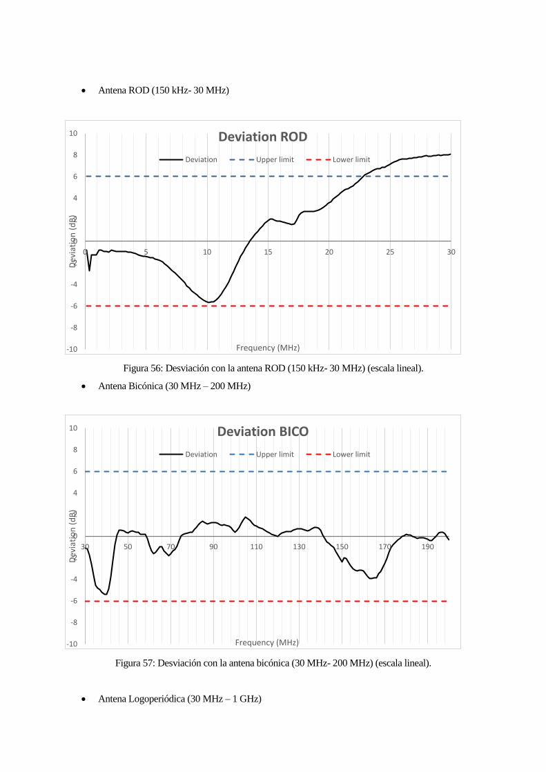
Antena ROD (150 kHz- 30 MHz)
Figura 56: Desviación con la antena ROD (150 kHz- 30 MHz) (escala lineal).
Antena Bicónica (30 MHz – 200 MHz)
Figura 57: Desviación con la antena bicónica (30 MHz- 200 MHz) (escala lineal).
Antena Logoperiódica (30 MHz – 1 GHz)
-10
-8
-6
-4
-2
0
2
4
6
8
10
0 5 10 15 20 25 30
Dev
iati
on
(d
B)
Frequency (MHz)
Deviation ROD
Deviation Upper limit Lower limit
-10
-8
-6
-4
-2
0
2
4
6
8
10
30 50 70 90 110 130 150 170 190
Dev
iati
on
(d
B)
Frequency (MHz)
Deviation BICO
Deviation Upper limit Lower limit

Figura 58: Desviación con la antena logo periódica (200 MHz- 1 GHz) (escala lineal).
Rango completo (150 kHz- 1 GHz)
Figura 59: Resultado de la desviación total (escala logarítmica).
Para calcular en qué tanto por ciento se cumple con la validación se utiliza la ecuación (2).
-10
-8
-6
-4
-2
0
2
4
6
8
10
200 300 400 500 600 700 800 900 1000
Dev
iati
on
(d
B)
Frequency (MHz)
Deviation LOGO
Deviation Upper limit Lower limit
-10
-8
-6
-4
-2
0
2
4
6
8
10
0,1 1 10 100 1000
Dev
iati
on
(d
B)
Frequency (MHz)
Deviation Max Min

(2)
Data points 150 kHz to 1000 MHz where Δlong wire method is within de ± 6 dB = 445
Total %IT 150 KHz to 1000 MHz, Long Wire Method= (445/481)*100= 92.52% ≥ al 90%
A la vista de los resultados obtenidos, con esta validación se concluye que la cámara cumple con los requisitos
del anexo J.
4 CONCLUSIONES
Como ya se indicó, el objetivo principal de este trabajo era plasmar una metodología para obtener una cámara
semianecoicas para componentes de automoción que cumpliese con las restricciones de la norma CISPR 25.
Primero se planteó el problema que existía en el laboratorio, la necesidad de ampliar éste para reducir los
tiempos de espera de los clientes y conseguir una mayor facturación. Ampliar el laboratorio pasaba por, entre
otras cosas, instalar una nueva cámara semianecoicas.
Una vez aprobado el proyecto se solicitó presupuesto a los principales proveedores de cámaras
semianecoicas. Finalmente se optó por algo distinto, reciclar una cámara que procedía del sector industrial,
aprovechando al máximo los materiales de los que se disponía e incorporando materiales nuevos cuando
fuera necesario. Este proyecto se llevaría a cabo conjuntamente con Albatross.
Tras el estudio de la planificación se realizó la construcción con personal de Albatross. A la vez, se
redimensionó la red eléctrica del edificio y se aisló la masa de las dos cámaras, SAC 3 y SAC 4, para que el
ruido procedente de los equipos electrónicos del resto del edificio no interfirieran en las medidas.
Cuando la obra concluyó, se realizó el test que validaría la cámara. El test se recoge en el anexo J de la
CISPR25 y proporciona dos métodos. Se escogió el método de antena modelada de cable largo y se puso en
práctica.
Los resultados de la medición se compararon con los resultados de referencia que proporciona el Anexo J y
aunque en algunas medidas existen desviaciones mayores del máximo requerido, el anexo J lo permite
siempre que se cumpla al menos con el 90% de las frecuencias medidas.
Se obtuvo un 92,52% de cumplimiento, con lo que la validación fue positiva.
Para finalizar se equipó la SAC con todo lo necesario para su puesta en marcha, equipos, cables,
monitorización… Actualmente, la SAC 4 es una cámara operativa para medidas de emisiones según la
CISPR25.
4.1 LINEAS FUTURAS
Durante los siguientes meses e incluso años después de la puesta en marcha de SAC4 será necesario realizarle
mejoras para cumplir con los cambios que surjan en la normativa o incluso en los equipos bajo prueba.
Durante las primeras semanas de funcionamiento se vio la necesidad de incluir una plataforma elevadora a
la entrada de la puerta para que sea mas facil meter y sacar equipos pesados de ella.
Por otra parte, para ciertos equipos es necesario el uso de aire comprimido, ya sea bien para refrijerar o para
activar algun mecanismo del propio EUT, de momento no se ha incorporado este mecanismo en SAC4 ya
que los equipos que lo han necesitado se han derivado a otras salas, pero se prevee incorporarlo en un futuro
para que SAC4 sea completamente autonoma.
ANEXOS

Dado el volumen de datos generados para la realización del presente estudio, se ha optado por incluir la
información más relevante en los anexos siguientes.
Anexo 1
CISPR25


CISPR/D/425A/CDV
COMMITTEE DRAFT FOR VOTE (CDV)
PROJET DE COMITÉ POUR VOTE (CDV) Project number CISPR 25 Ed. 4 Numéro de projet IEC/TC or SC: CISPR/D CEI/CE ou SC:
Secretariat / Secrétariat Germany
Submitted for parallel voting in CENELEC Soumis au vote parallèle au CENELEC
Date of circulation Date de diffusion 2015-02-20
Closing date for voting (Voting mandatory for P-members) Date de clôture du vote (Vote obligatoire pour les membres (P)) 2015-05-15*
Also of interest to the following committees Intéresse également les comités suivants CISPR/A, TC69
Supersedes document Remplace le document CISPR/D/419/CD, CISPR/D/424/CC
Proposed horizontal standard Norme horizontale suggérée
Other TC/SCs are requested to indicate their interest, if any, in this CDV to the TC/SC secretary Les autres CE/SC sont requis d’indiquer leur intérêt, si nécessaire, dans ce CDV à l’intention du secrétaire du CE/SC Functions concerned Fonctions concernées
Safety Sécurité
EMC CEM
Environment Environnement
Quality assurance Assurance qualité
CE DOCUMENT EST TOUJOURS À L'ÉTUDE ET SUSCEPTIBLE DE MODIFICATION. IL NE PEUT SERVIR DE RÉFÉRENCE.
LES RÉCIPIENDAIRES DU PRÉSENT DOCUMENT SONT INVITÉS À PRÉSENTER, AVEC LEURS OBSERVATIONS, LA NOTIFICATION DES DROITS DE PROPRIÉTÉ DONT ILS AURAIENT ÉVENTUELLEMENT CONNAISSANCE ET À FOURNIR UNE DOCUMENTATION EXPLICATIVE.
THIS DOCUMENT IS STILL UNDER STUDY AND SUBJECT TO CHANGE. IT SHOULD NOT BE USED FOR REFERENCE PURPOSES.
RECIPIENTS OF THIS DOCUMENT ARE INVITED TO SUBMIT, WITH THEIR COMMENTS, NOTIFICATION OF ANY RELEVANT PATENT RIGHTS OF WHICH THEY ARE AWARE AND TO PROVIDE SUPPORTING DOCUMENTATION.
Titre : CISPR 25: Véhicules, bateaux et moteurs á combustion interne - Caractéristique des pertubations radioélectriques - Limites et méthodes de mesure pour la protection des récepteurs embarqués
Title : CISPR 25: Vehicles, boats and internal combustion engines - Radio disturbance characteristics - Limits and methods of measurement for the protection of on-board receivers
Introductory note This draft contains test methods for vehicles in charging mode as well as specific methods needed to test components for a shielded high voltage board net as used in electric and hybrid electric vehicles. It also contains the results of the CISPR/D-CISPR/A-project on chamber validation for ALSEs used for component testing.
*IEC CO Note: Please be informed that an “A” version of the CDV is circulated due to a problem which occurred in the document during the pdf conversion with some figures and the formatting of the document. The closing date for voting remains unchanged.
ATTENTION
VOTE PARALLÈLE IEC – CENELEC
L’attention des Comités nationaux de l’IEC, membres du CENELEC, est attirée sur le fait que ce projet de comité pour vote (CDV) de Norme internationale est soumis au
vote parallèle. Les membres du CENELEC sont invités à voter via le
système de vote en ligne du CENELEC.
ATTENTION IEC – CENELEC
PARALLEL VOTING The attention of IEC National Committees, members of
CENELEC, is drawn to the fact that this Committee Draft for Vote (CDV) for an International Standard is submitted for
parallel voting. The CENELEC members are invited to vote through the
CENELEC online voting system.
Copyright © 2015 International Electrotechnical Commission, IEC. All rights reserved. It is permitted to download this electronic file, to make a copy and to print out the content for the sole purpose of preparing National Committee positions. You may not copy or "mirror" the file or printed version of the document, or any part of it, for any other purpose without permission in writing from IEC.
®

CISPR CDV 25 IEC 2014 – 2 – CISPR/D/425A/CDV
CONTENTS
FOREWORD .......................................................................................................................... 9 INTRODUCTION .................................................................................................................. 11 1 Scope ........................................................................................................................... 12 2 Normative references .................................................................................................... 13 3 Definitions..................................................................................................................... 14 4 Requirements common to vehicle and component/module emissions measurement ...... 20
4.1 General test requirements and test plan .......................................................... 20 4.1.1 Categories of disturbance sources (as applied in the test plan) ...... 20 4.1.2 Test plan ........................................................................................ 20 4.1.3 Determination of conformance of equipment under test (EUT) with limits
...................................................................................................... 20 4.1.4 Operating conditions ...................................................................... 22 4.1.5 Test report ..................................................................................... 22
4.2 Shielded enclosure .......................................................................................... 22 4.3 Absorber-lined shielded enclosure (ALSE) ...................................................... 22
4.3.1 Size ............................................................................................... 23 4.3.2 Objects in ALSE ............................................................................. 23 4.3.3 ALSE performance validation ......................................................... 23
4.4 Measuring instrument ...................................................................................... 23 4.4.1 Spectrum analyser parameters ....................................................... 23 4.4.2 Scanning receiver parameters ........................................................ 24
4.5 Power supply .................................................................................................. 27 5 Measurement of emissions received by an antenna on the same vehicle ...................... 28
5.1 Antenna measuring system ............................................................................. 28 5.1.1 Type of antenna ............................................................................. 28 5.1.2 Measuring system requirements ..................................................... 29
5.2 Method of measurement .................................................................................. 30 5.3 Test setup for vehicle in charging mode .......................................................... 32
5.3.1 a.c. power charging without communication ................................... 32 5.3.2 a.c. or d.c. power charging with communication line(s) or with signal
line(s) ............................................................................................ 35 5.4 Examples of limits for vehicle radiated disturbances ........................................ 40
6 Measurement of components and modules ................................................................... 44 6.1 General ........................................................................................................... 44 6.2 Test equipment ............................................................................................... 44
6.2.1 Reference ground plane ................................................................. 44 6.2.2 Power supply and AN ..................................................................... 44 6.2.3 Load Simulator ............................................................................... 45 6.2.4 Signal/control line filters ................................................................. 45
6.3 Conducted emissions from components/modules – Voltage method ................ 46 6.3.1 General .......................................................................................... 46

CISPR CDV 25 IEC 2014 – 3 – CISPR/D/425A/CDV
6.3.2 Reference ground plane arrangement ............................................ 47 6.3.3 Limits for conducted disturbances from components/modules – Voltage
method ........................................................................................... 55 6.4 Conducted emissions from components/modules – current probe method ....... 57
6.4.1 Test setup ...................................................................................... 57 6.4.2 Test procedure ............................................................................... 57 6.4.3 Limits for conducted disturbances from components/modules – Current
probe method ................................................................................. 60 6.5 Radiated emissions from components/modules - ALSE method ....................... 61
6.5.1 General .......................................................................................... 61 6.5.2 Test setup ...................................................................................... 61 6.5.3 Test procedure ............................................................................... 65 6.5.4 Limits for radiated disturbances from components/modules – ALSE
method ........................................................................................... 71 6.6 Radiated emissions from components/modules – TEM cell method ................. 73 6.7 Radiated emissions from components/modules – Stripline method .................. 74
Annex A (informative) Flow chart for checking the applicability of CISPR 25 ....................... 75 Annex B (normative) Antenna matching unit – Vehicle test .................................................. 76
B.1 Antenna matching unit parameters (150 kHz to 6,2 MHz) ................................ 76 B.2 Antenna matching unit – verification ................................................................ 76
B.2.1 Gain measurement ......................................................................... 76 B.2.2 Test procedure ............................................................................... 76
B.3 Impedance measurement ................................................................................ 76 Annex C (informative) Sheath-current suppressor ............................................................... 78
C.1 General Information ........................................................................................ 78 C.2 Suppressor Construction ................................................................................. 78
Annex D (informative) Guidance for the determination of the noise floor of active vehicle antennas in the AM and FM Range ............................................................................... 80
Annex E (normative) Artificial Networks (AN), Artificial Mains Networks (AMN) and Asymmetric Artificial Networks (AAN) ............................................................................................... 85 E.1 General ........................................................................................................... 85 E.2 Artificial networks (AN) .................................................................................... 85
E.2.1 Component powered by LV ............................................................ 85 E.2.2 Component powered by HV ............................................................ 87 E.2.3 Component involved in charging mode connected to d.c. power mains
...................................................................................................... 90 E.2.4 Vehicle in charging mode connected to d.c. power mains ............... 90
E.3 Artificial Mains networks (AMN) ....................................................................... 90 E.3.1 Component AMN ............................................................................ 90 E.3.2 Vehicle in charging mode connected to a.c. power mains ............... 90
E.4 Asymmetric artificial network (AAN):................................................................ 90 E.4.1 Symmetric communication lines ..................................................... 90 E.4.2 PLC on power lines ........................................................................ 91 E.4.3 PLC (technology) on control pilot ................................................... 92
Annex F (informative) Radiated emissions from components/modules – TEM cell method ... 94

CISPR CDV 25 IEC 2014 – 4 – CISPR/D/425A/CDV
F.1 General ........................................................................................................... 94 F.2 Test setup ....................................................................................................... 95
F.2.1 Setup with major field emission from the wiring harness ................. 95 F.2.2 Setup with major field emissions from the EUT............................... 97
F.3 Test procedure ................................................................................................ 97 F.4 Limits for radiated disturbances from components/modules – TEM cell method 98 F.5 TEM Cell design .............................................................................................. 99
Annex G (informative) Radiated emissions from components/modules – Stripline method . 102 G.1 General ......................................................................................................... 102 G.2 Test setup ..................................................................................................... 102
G.2.1 Stripline impedance matching ...................................................... 102 G.2.2 Location of the EUT ..................................................................... 103 G.2.3 Location and length of the test harness ........................................ 103 G.2.4 Location of the load simulator ...................................................... 103
G.3 Test procedure .............................................................................................. 103 G.4 Limits for radiated emissions from components/modules – Stripline method .. 105 G.5 Stripline design ............................................................................................. 107
Annex H (informative) Interference to mobile radio communication in the presence of impulsive noise – Methods of judging degradation ...................................................................... 111 H.1 Introduction ................................................................................................... 111 H.2 Survey of methods of judging degradation to radio channel ........................... 111
H.2.1 Subjective tests............................................................................ 111 H.2.2 Objective tests ............................................................................. 113 H.2.3 Conclusions relating to judgement of degradation ........................ 113
H.3 Bibliography .................................................................................................. 114 Annex I (normative) Test methods for shielded power supply systems for high voltages in
electric and hybrid vehicles ......................................................................................... 115 I.1 General ......................................................................................................... 115 I.2 Conducted emission from components/modules on HV power lines – Voltage
method .......................................................................................................... 116 I.2.1 Ground plane arrangement .......................................................... 116 I.2.2 Test set-up ................................................................................... 116 I.2.3 Limits for conducted emission – Voltage method .......................... 121
I.3 Conducted emission from components/modules on HV power lines – current probe method .......................................................................................................... 123 I.3.1 Ground plane arrangement .......................................................... 123 I.3.2 Test setup .................................................................................... 123 I.3.3 Limits for conducted emission – current probe method ................. 128
I.4 Radiated emissions from components/modules – ALSE method .................... 128 I.4.1 Ground plane arrangement .......................................................... 128 I.4.2 Test setup .................................................................................... 128 I.4.3 Limits for radiated emissions – ALSE method ............................... 133
I.5 Coupling between HV and LV systems .......................................................... 133 I.5.1 General ........................................................................................ 133

CISPR CDV 25 IEC 2014 – 5 – CISPR/D/425A/CDV
I.5.2 Measurement based on CISPR 25 test setup defined in the main part .................................................................................................... 133
I.5.3 Measurement of the HV-LV Scattering parameters ....................... 140 Annex J (informative) ALSE Performance Validation 150 kHz – 1 GHz .............................. 144
J.1 Introduction ................................................................................................... 144 J.1.1 Purpose ....................................................................................... 146 J.1.2 Repetition period of ALSE validation measurements ..................... 146
J.2 Reference measurement method ................................................................... 146 J.2.1 Overview ...................................................................................... 146 J.2.2 Equipment .................................................................................... 147 J.2.3 Procedure .................................................................................... 148 J.2.4 Requirements ............................................................................... 153
J.3 Modelled long wire antenna method .............................................................. 153 J.3.1 Overview ...................................................................................... 153 J.3.2 Equipment .................................................................................... 154 J.3.3 Procedure .................................................................................... 156 J.3.4 Requirements ............................................................................... 164
J.4 References .................................................................................................... 166 Annex K (informative) Items Under Consideration ............................................................. 167
K.1 Introduction ................................................................................................... 167 K.1.1 Measurement techniques and limits ............................................. 167 K.1.2 Measurement Uncertainty ............................................................ 167
Figure 1 – Method of determination of conformance for all frequency bands ......................... 21 Figure 2 – Example of gain curve ......................................................................................... 29 Figure 3 –Vehicle-radiated emissions – Example for test layout (end view with monopole antenna) .............................................................................................................................. 31 Figure 4 – Example of test setup for vehicle with plug located on vehicle side (a.c. powered without communication) ........................................................................................................ 33 Figure 5 – Example of test setup for vehicle with plug located front / rear of vehicle (a.c. powered without communication) ........................................................................................................ 35 Figure 6 – Example of test setup for vehicle with plug located on vehicle side (a.c. or d.c. powered with communication) .............................................................................................. 38 Figure 7 – Example of test setup for vehicle with plug located front /rear of vehicle (a.c. or d.c. powered with communication) .............................................................................................. 40 Figure 8a – Average limit for radiated disturbances from vehicles GPS band 1 567,42 to 1 583,42 MHz ....................................................................................................................... 42 Figure 8b – Average limit for radiated disturbance from vehicles GLONASS band 1 591,065 to 1 613,5 MHz ......................................................................................................................... 43 Figure 9 – Example for the required minimum attenuation of the Signal / Control line filters . 46 Figure 10 – Setup for measurement of the filter attenuation ................................................. 46 Figure 11 – Conducted emissions – Example of test setup for EUT with power return line remotely grounded. .............................................................................................................. 49 Figure 12 – Conducted emissions – Example of test setup for EUT with power return line locally grounded .............................................................................................................................. 50

CISPR CDV 25 IEC 2014 – 6 – CISPR/D/425A/CDV Figure 13 – Conducted emissions – Example of test setup for alternators and generators .... 52 Figure 14 – Conducted emissions – Example of test setup for ignition system components .. 54 Figure 15– Conducted emissions – Example of test setup for current probe measurements 59 Figure 16 – Test harness bending requirements ................................................................... 64 Figure 17 – Example of test setup – rod antenna .................................................................. 67 Figure 18 – Example of test setup – biconical antenna ......................................................... 68 Figure 19 – Example of test setup – log-periodic antenna .................................................... 70 Figure 20 – Example of test setup – above 1 GHz ................................................................ 71 Figure 21a – Example of average limit for radiated disturbances from components GPS band 1 567,42 to 1 583,42 MHz .................................................................................................... 73 Figure 21b – Example of average limit for radiated disturbances from components GLONASS band 1 591,065 MHz to 1 613,5 MHz .................................................................................... 73 Figure B.1 –Verification setup .............................................................................................. 77 Figure C.1 – Characteristic S21 of the ferrite core ................................................................. 79 Figure D.1 – Vehicle test setup for equipment noise measurement in the AM/FM range ....... 82 Figure D.2 - Vehicle test setup for antenna noise measurement in the AM/FM range ............ 84 Figure E.1 – Example of 5 mH AN schematic ........................................................................ 86 Figure E.2 – Characteristics of the AN impedance ZPB ......................................................... 86
Figure E.3 – Example of 5 mH HV AN schematic .................................................................. 88 Figure E.4 – Characteristics of the HV AN impedance .......................................................... 88 Figure E.5 – Example of 5 mH HV AN combination in a single shielded box .......................... 89 Figure E.6 – Impedance matching network attached between HV ANs and EUT ................... 90 Figure E.7 Example of an AAN for symmetric communication lines....................................... 91 Figure E.8 Example of AAN circuit of PLC on a.c. or d.c. powerlines .................................... 92 Figure E.9 Example of AAN circuit for PLC on pilot line ........................................................ 93 Figure F.1 - TEM cell (example) ........................................................................................... 94 Figure F.2 – Example of arrangement of leads in the TEM cell and to the connector panel .. 96 Figure F.3 – Example of the arrangement of the connectors, the lead frame and the dielectric support ................................................................................................................................. 96 Figure F.4 – Example of the TEM cell method test setup ...................................................... 97 Figure F.5 – TEM cell ......................................................................................................... 101 Figure G.1 – Example of a basic stripline test setup in a shielded enclosure ...................... 105 Figure G.2 – Example for a 50 Ω stripline ........................................................................... 108 Figure G.3 – Example for a 90 Ω stripline ........................................................................... 110 Figure I.1 – Conducted emission – example for test setup for EUTs with shielded power supply systems.............................................................................................................................. 119 Figure I.2 – Conducted emission – example of test setup for EUTs with shielded power supply systems with electric motor attached to the bench .............................................................. 120 Figure I.3 – Conducted emission - example of test setup for EUTs with shielded power supply systems and inverter/charger device .................................................................................. 121

CISPR CDV 25 IEC 2014 – 7 – CISPR/D/425A/CDV Figure I.4 – Conducted emission - example of test setup current probe measurement on HV lines for EUTs with shielded power supply systems .................................................................... 126 Figure I.5 – Conducted emission - example of test setup current probe measurement on HV lines for EUTs with shielded power supply systems with electric motor attached to the bench .... 127 Figure I.6 – Conducted emission - example of test setup current probe measurement on HV lines for EUTs with shielded power supply systems and inverter/charger device ......................... 128 Figure I.7 – Radiated emission - example of test setup measurement with biconical antenna for EUTs with shielded power supply systems ......................................................................... 131 Figure I.8 – Radiated emission - example of test setup measurement with biconical antenna for EUTs with shielded power supply systems with electric motor attached to the bench ......... 132 Figure I.9 – Radiated emission - example of test setup measurement with biconical antenna for EUTs with shielded power supply systems and inverter/charger device .............................. 133 Figure I.10 – Test setup for calibration of the test signal .................................................... 135 Figure I.11 – Conducted emission – test setup for measurement decoupling factor between HV supply ports and LV port .................................................................................................... 137 Figure I.12 – Conducted emission - test setup for measurement decoupling factor between HV supply ports and LV ports with current probe ...................................................................... 138 Figure I.13 – Radiated emission - test setup measurement decoupling factor between HV supply ports and LV ports with biconical antenna .......................................................................... 140 Figure I.14 – Test setup for EUT measurements................................................................. 141 Figure I.15 – Examples of requirements for S21EUT. ............................................................. 143 Figure J.1 – ALSE influence parameters over the 10 – 100 MHz frequency range .............. 145 Figure J.2 – Visual Representation of ALSE Performance Validation Process ..................... 146 Figure J.3 – Example of construction of a transmitting monopole ....................................... 148 Figure J.4 – Side view of antenna configuration for reference measurement below 30 MHz 150 Figure J.5 – Top view of antenna configuration for reference measurement 30 MHz and above (with the biconical antenna shown as example) .................................................................. 151 Figure J.6 – Side view of antenna configuration for reference measurement 30 MHz and above (with the biconical antenna shown as example) .................................................................. 151 Figure J.7 – Top view of antenna configuration for the ALSE measurement below 30 MHz . 152 Figure J.8 - Metallic sheet angles used as support for the rod ............................................ 155 Figure J.9 - Radiator side view 50 Ω terminations .............................................................. 155 Figure J.10 - Photo of the radiator mounted on the ground reference plane ........................ 155 Figure J.11 - Example VSWR measured from four radiation sources (without 10 dB) .......... 156 Figure J.12 - Example setup for ALSE equivalent field strength measurement (rod antenna shown for the frequency range below 30 MHz). .................................................................. 158 Figure J.13 - MoM-Modell for the frequency range 30MHz to 200 MHz ............................... 159 Table 1 – Spectrum analyser parameters ............................................................................. 25 Table 2 – Scanning receiver parameters .............................................................................. 27 Table 3 – Antenna types ...................................................................................................... 28 Table 4 – Example for limits of disturbance – Complete vehicle............................................ 41 Table 5 – Examples of limits for conducted disturbances – Voltage Method ........................ 56

CISPR CDV 25 IEC 2014 – 8 – CISPR/D/425A/CDV Table 6 – Examples of limits for conducted disturbances - control/signal lines – Current probe method ................................................................................................................................. 60 Table 7 – Examples of Limits for radiated disturbances – ALSE method ............................... 72 Table E.1 Magnitude of the AN impedance ZPB ................................................................... 87 Table F.1 – Examples of limits for radiated disturbances – TEM cell method ........................ 99 Table F.2 – Dimensions for TEM cells ................................................................................ 101 Table G.1 – Examples of limits for radiated disturbances – Stripline method ..................... 106 Table I.1 – Example for limits for conducted voltage measurements at shielded power supply devices .............................................................................................................................. 122 Table I.2 – Configurations for equipment without negative LV line ...................................... 141 Table I.3 – Configurations for equipment with negative LV line ........................................... 142 Table I.4 – Examples of requirements for S21EUT ................................................................. 142 Table J.1 Reference data to be used for chamber validation ............................................... 160

CISPR CDV 25 IEC 2014 – 9 – CISPR/D/425A/CDV
INTERNATIONAL ELECTROTECHNICAL COMMISSION 1 2
INTERNATIONAL SPECIAL COMMITTEE ON RADIO INTERFERENCE 3
____________ 4 5 6
VEHICLES, BOATS AND INTERNAL COMBUSTION ENGINES – 7 RADIO DISTURBANCE CHARACTERISTICS – 8
LIMITS AND METHODS OF MEASUREMENT FOR THE PROTECTION OF ON-9 BOARD RECEIVERS 10
11 12 13
FOREWORD 14
1) The International Electrotechnical Commission (IEC) is a worldwide organization for standardization comprising all national 15 electrotechnical committees (IEC National Committees). The object of IEC is to promote international co-operation on all 16 questions concerning standardization in the electrical and electronic fields. To this end and in addition to other activities, 17 IEC publishes International Standards, Technical Specifications, Technical Reports, Publicly Available Specifications (PAS) 18 and Guides (hereafter referred to as “IEC Publication(s)”). Their preparation is entrusted to technical committees; any IEC 19 National Committee interested in the subject dealt with may participate in this preparatory work. International, governmental 20 and non-governmental organizations liaising with the IEC also participate in this preparation. IEC collaborates closely with 21 the International Organization for Standardization (ISO) in accordance with conditions determined by agreement between 22 the two organizations. 23
2) The formal decisions or agreements of IEC on technical matters express, as nearly as possible, an international consensus 24 of opinion on the relevant subjects since each technical committee has representation from all interested IEC National 25 Committees. 26
3) IEC Publications have the form of recommendations for international use and are accepted by IEC National Committees in 27 that sense. While all reasonable efforts are made to ensure that the technical content of IEC Publications is accurate, IEC 28 cannot be held responsible for the way in which they are used or for any misinterpretation by any end user. 29
4) In order to promote international uniformity, IEC National Committees undertake to apply IEC Publications transparently to 30 the maximum extent possible in their national and regional publications. Any divergence between any IEC Publication and 31 the corresponding national or regional publication shall be clearly indicated in the latter. 32
5) IEC itself does not provide any attestation of conformity. Independent certification bodies provide conformity assessment 33 services and, in some areas, access to IEC marks of conformity. IEC is not responsible for any services carried out by 34 independent certification bodies. 35
6) All users should ensure that they have the latest edition of this publication. 36 7) No liability shall attach to IEC or its directors, employees, servants or agents including individual experts and members of 37
its technical committees and IEC National Committees for any personal injury, property damage or other damage of any 38 nature whatsoever, whether direct or indirect, or for costs (including legal fees) and expenses arising out of the publication, 39 use of, or reliance upon, this IEC Publication or any other IEC Publications. 40
8) Attention is drawn to the Normative references cited in this publication. Use of the referenced publications is indispensable 41 for the correct application of this publication. 42
9) Attention is drawn to the possibility that some of the elements of this IEC Publication may be the subject of patent rights. 43 IEC shall not be held responsible for identifying any or all such patent rights. 44
International Standard CISPR 25 has been prepared by CISPR subcommittee D: Electromagnetic 45 disturbances related to electric/electronic equipment on vehicles and internal combustion engine 46 powered devices. 47
This fourth edition cancels and replaces the third edition published in 2008. This edition constitutes a 48 technical revision. 49

CISPR CDV 25 IEC 2014 – 10 – CISPR/D/425A/CDV The following significant changes were made with respect to the previous edition: 50
• inclusion of charging mode for EV and PHEV, 51
• overall improvement 52
• the methods for chamber validation have been included 53
• test methods for shielded power supply systems for high voltages for electric and hybrid electric 54 vehicles have been included 55
The text of this standard is based on the following documents: 56
FDIS Report on voting
XX/XX/FDIS XX/XX/RVD
57 Full information on the voting for the approval of this standard can be found in the report on voting 58 indicated in the above table. 59
This publication has been drafted in accordance with the ISO/IEC Directives, Part 2. 60
The committee has decided that the contents of this publication will remain unchanged until the stability 61 date indicated on the IEC web site under "http://webstore.iec.ch" in the data related to the specific 62 publication. At this date, the publication will be 63
• reconfirmed, 64
• withdrawn, 65
• replaced by a revised edition, or 66
• amended. 67 68
The National Committees are requested to note that for this publication the stability date is 2020. 69
THIS TEXT IS INCLUDED FOR THE INFORMATION OF THE NATIONAL COMMITTEES AND WILL BE DELETED AT THE 70 PUBLICATION STAGE. 71
72

CISPR CDV 25 IEC 2014 – 11 – CISPR/D/425A/CDV
INTRODUCTION 73
This International Standard is designed to protect on-board receivers from disturbances produced by 74 conducted and radiated emissions arising in a vehicle. 75
Test procedures and limits given are intended to provide provisional control of vehicle radiated 76 emissions, as well as component/module conducted/radiated emissions of long and short duration. 77
To accomplish this end, this standard: 78
• establishes a test method for measuring the electromagnetic emissions from the electrical 79 system of a vehicle; 80
• sets limits for the electromagnetic emissions from the electrical system of a vehicle; 81
• establishes test methods for testing on-board components and modules independent from the 82 vehicle; 83
• sets limits for electromagnetic emissions from components to prevent objectionable disturbance 84 to on-board receivers; 85
• classifies automotive components by disturbance duration to establish a range of limits. 86 87 NOTE Component tests are not intended to replace vehicle tests. Exact correlation between component and vehicle test performance is 88 dependent on component mounting location, harness length, routing and grounding, as well as antenna location. Component testing, 89 however, permits components to be evaluated prior to actual vehicle availability. 90
91
92

CISPR CDV 25 IEC 2014 – 12 – CISPR/D/425A/CDV 93
94 VEHICLES, BOATS AND INTERNAL COMBUSTION ENGINES – 95
RADIO DISTURBANCE CHARACTERISTICS – 96 LIMITS AND METHODS OF MEASUREMENT FOR 97 THE PROTECTION OF ON-BOARD RECEIVERS 98
99 100 101
1 Scope 102
This International Standard contains limits and procedures for the measurement of radio disturbances in 103 the frequency range of 150 kHz to 2 500 MHz. The standard applies to any electronic/electrical 104 component intended for use in vehicles, trailers and devices. Refer to International Telecommunications 105 Union (ITU) publications for details of frequency allocations. The limits are intended to provide 106 protection for receivers installed in a vehicle from disturbances produced by components/modules in the 107 same vehicle. The method and limits for a complete vehicle (whether connected to the power mains for 108 charging purposes or not) are in Clause 5 and the methods and limits for components/modules are in 109 Clause 6. Only a complete vehicle test can be used to determine the component compatibility with 110 respect to a vehicle’s limit. 111
The receiver types to be protected are, for example, broadcast receivers (sound and television), land 112 mobile radio, radio telephone, amateur, citizens' radio, Satellite Navigation (GPS etc.) and Bluetooth. 113 For the purpose of this standard, a vehicle is a machine, which is self-propelled by an internal 114 combustion engine, electric means, or both. Vehicles include (but are not limited to) passenger cars, 115 trucks, agricultural tractors and snowmobiles. Annex A provides guidance in determining whether this 116 standard is applicable to particular equipment. 117
The limits in this standard are recommended and subject to modification as agreed between the vehicle 118 manufacturer and the component supplier. This standard is also intended to be applied by manufactur-119 ers and suppliers of components and equipment which are to be added and connected to the vehicle 120 harness or to an on-board power connector after delivery of the vehicle. 121
This International Standard does not include protection of electronic control systems from radio 122 frequency (RF) emissions, or from transient or pulse-type voltage fluctuations. These subjects are 123 included in ISO publications. 124
Since the mounting location, vehicle body construction and harness design can affect the coupling of 125 radio disturbances to the on-board radio, Clause 6 of this standard defines multiple limit levels. The 126 level class to be used (as a function of frequency band) shall be agreed upon between the vehicle 127 manufacturer and the component supplier. 128
CISPR 25 defines test methods for use by Vehicle Manufacturers and Suppliers, to assist in the design 129 of vehicles and components and ensure controlled levels of on-board radio frequency emissions. 130
Vehicle test limits are provided for guidance and are based on a typical radio receiver using the antenna 131 provided as part of the vehicle, or a test antenna if a unique antenna is not specified. The frequency 132 bands that are defined are not applicable to all regions or countries of the world. For economic reasons, 133 the vehicle manufacturer must be free to identify what frequency bands are applicable in the countries 134 in which a vehicle will be marketed and which radio services are likely to be used in that vehicle. 135

CISPR CDV 25 IEC 2014 – 13 – CISPR/D/425A/CDV As an example, many vehicle models will probably not have a television receiver installed; yet the 136 television bands occupy a significant portion of the radio spectrum. Testing and mitigating noise sources 137 in such vehicles is not economically justified. 138
The vehicle manufacturer should define the countries in which the vehicle is to be marketed, then 139 choose the applicable frequency bands and limits. Component test parameters can then be selected 140 from CISPR 25 to support the chosen marketing plan. 141
The World Administrative Radio communications Conference (WARC) lower frequency limit in region 1 142 was reduced to 148,5 kHz in 1979. For vehicular purposes, tests at 150 kHz are considered adequate. 143 For the purposes of this standard, test frequency ranges have been generalized to cover radio services 144 in various parts of the world. Protection of radio reception at adjacent frequencies can be expected in 145 most cases. 146
Annex E defines artificial networks used for the measurement of conducted disturbances and for tests 147 on vehicles in charging mode. 148
Annex H defines a qualitative method of judging the degradation of radio communication in the 149 presence of impulsive noise. 150
Annex I defines test methods for shielded power supply systems for high voltage networks in electric 151 and hybrid vehicles. 152
Annex J defines methods for the validation of the ALSE and the reference ground plane used for 153 component testing. 154
Annex K lists work being considered for future revisions. 155
2 Normative references 156
The following referenced documents are indispensable for the application of this document. For dated 157 references, only the edition cited applies. For undated references, the latest edition of the referenced 158 document (including any amendments) applies 159
IEC 60050-161:1990, International Electrotechnical Vocabulary (IEV) – Chapter 161: Electromagnetic 160 compatibility 161 Amendment 1 (1997) 162 Amendment 2 (1998) 163 Amendment 3 (2014) 164 Amendment 4 (2014) 165
CISPR 12:2009, Vehicles, motorboats, and internal combustion engine-driven devices – Radio 166 disturbance characteristics - Limits and methods of measurement for the protection of receivers except 167 those installed in the vehicle/boat/device itself or in adjacent vehicles/boats/devices 168
CISPR 16-1-1:2010, Specification for radio disturbance and immunity measuring apparatus and 169 methods – Part 1-1: Radio disturbance and immunity measuring apparatus – Measuring apparatus 170 Amendment 1 (2010) 171 Amendment 2 (2014) 172

CISPR CDV 25 IEC 2014 – 14 – CISPR/D/425A/CDV CISPR 16-1-2:2014, Specification for radio disturbance and immunity measuring apparatus and 173 methods - Part 1-2: Radio disturbance and immunity measuring apparatus - Ancillary equipment - 174 Conducted disturbances 175
176 CISPR 16-1-4:2010, Specification for radio disturbance and immunity measuring apparatus and 177 methods - Part 1-4: Radio disturbance and immunity measuring apparatus - Ancillary equipment - 178 Radiated disturbances 179 Amendment 1 (2012) 180
CISPR 16-2-1:2014, Specification for radio disturbance and immunity measuring apparatus and 181 methods - Part 2-1: Methods of measurement of disturbances and immunity - Conducted disturbance 182 measurements 183
CISPR 16-2-3:2010, Specification for radio disturbance and immunity measuring apparatus and 184 methods - Part 2-3: Methods of measurement of disturbances and immunity - Radiated disturbance 185 measurements 186 Amendment 1 (2010) 187 Amendment 2 (2014) 188
ISO 11452-4:2011, Road vehicles — Component test methods for electrical disturbances from 189 narrowband radiated electromagnetic energy — Part 4: Bulk current injection (BCI) 190
SAE ARP 958.1 Rev D: 2003-02 - Electromagnetic Interference Measurement Antennas; Standard 191 Calibration Method 192
3 Definitions 193
For the purpose of this International Standard, the following definitions apply. 194
3.1 195 absorber lined shielded enclosure (ALSE) 196 shielded enclosure/screened room with radio frequency-absorbing material on its internal ceiling and 197 walls 198
3.2 199 antenna factor 200 the factor which is applied to the voltage measured at the input connector of the measuring instrument 201 to give the field strength at the antenna 202
3.3 203 antenna matching unit 204 a unit for matching the impedance of an antenna to that of the 50 Ω measuring instrument over the 205 antenna measuring frequency range 206
3.4 207 class 208 a performance level agreed upon by the purchaser and the supplier and documented in the test plan 209
3.5 210 component continuous conducted emissions 211 the noise voltages/currents of a steady-state nature existing on the supply or other leads of a 212 component/module which may cause disturbance to reception in an on-board receiver 213

CISPR CDV 25 IEC 2014 – 15 – CISPR/D/425A/CDV 3.6 214 compression point 215 the input signal level at which the gain of the measuring system becomes non-linear such that the 216 indicated output deviates from an ideal linear receiving system's output by the specified increment in dB 217
218

CISPR CDV 25 IEC 2014 – 16 – CISPR/D/425A/CDV 3.7 219 device 220 a machine driven by an internal combustion engine which is not primarily intended to carry persons or 221 goods 222
Note devices include, but are not limited to, chainsaws, irrigation pumps, snow blowers, air compressors, and landscaping 223 equipment. 224
3.8 225 receiver terminal voltage (antenna voltage) 226 the voltage generated by a source of radio disturbance and measured in dB(mV) by a radio disturbance 227 measuring instrument conforming to the requirements of CISPR 16 228
3.9 229 RF boundary 230 an element of an EMC test setup that determines what part of the harness and/or peripherals are 231 included in the RF environment and what is excluded. It may consist of, for example, ANs, filter feed-232 through pins, RF absorber coated wire, and/or RF shielding. 233
3.10 234 artificial network (AN) 235 a network inserted in the supply lead or signal/load lead of apparatus to be tested which provides, in a 236 given frequency range, a specified load impedance for the measurement of disturbance voltages and 237 which may isolate the apparatus from the supply or signal sources/loads in that frequency range 238
Note network inserted in the d.c power lines of the vehicle in charging mode which provides, in a given frequency range, a 239 specified load impedance and which isolates the vehicle from the d.c power supply in that frequency range” 240
3.11 241 average detector 242 a detector, the output voltage of which is the average value of the envelope of an applied signal 243
Note The average value must be taken over a specified time interval. 244
[IEV 161-04-26] 245
3.12 246 bandwidth 247
248 bandwidth (of an equipment) 249 the width of a frequency band over which a given characteristic of an equipment or transmission 250 channel does not differ from its reference value by more than a specified amount or ratio 251
Note The given characteristic may be, for example, the amplitude/frequency characteristic, the phase/frequency characteristic 252 or the delay/frequency characteristic. 253
[IEV 161-06-09, modified] 254
bandwidth (of an emission or signal) 255 the width of the frequency band outside which the level of any spectral component does not exceed a 256 specified percentage of a reference level 257
[IEV 161-06-10] 258
259

CISPR CDV 25 IEC 2014 – 17 – CISPR/D/425A/CDV 3.13 260 broadband emission 261 an emission which has a bandwidth greater than that of a particular measuring apparatus or receiver 262
Note An emission which has a pulse repetition rate (in Hz) less than the bandwidth of a particular measuring instrument can 263 also be considered as a broadband emission. 264
[IEV 161-06-11, modified] 265
3.14 266 disturbance suppression 267 action which reduces or eliminates electromagnetic disturbance 268
[IEV 161-03-22] 269
3.15 270 disturbance voltage; interference voltage (deprecated in this sense) 271 voltage produced between two points on two separate conductors by an electromagnetic disturbance, 272 measured under specified conditions 273
[IEV 161-04-01] 274
3.16 275 electromagnetic environment 276 the totality of electromagnetic phenomena existing at a given location 277
[IEV 161-01-01] 278
3.17 279 reference ground plane 280 a flat conductive surface whose potential is used as a common reference. 281 282 Note For the purpose of this standard, the reference ground plane is defined as the top metallic surface of the test bench/table. 283
[IEV 161-04-36] 284
3.18 285 narrowband emission 286 an emission which has a bandwidth less than that of a particular measuring apparatus or receiver 287
Note An emission which has a pulse repetition rate (in Hz) greater than the bandwidth of a particular measuring instrument can 288 also be considered as a narrowband emission. 289
[IEV 161-06-13] 290
3.19 291 peak detector 292 a detector, the output voltage of which is the peak value of an applied signal 293
[IEV 161-04-24] 294
295

CISPR CDV 25 IEC 2014 – 18 – CISPR/D/425A/CDV 3.20 296 quasi-peak detector 297 a detector having specified electrical time constants which, when regularly repeated identical pulses are 298 applied to it, delivers an output voltage which is a fraction of the peak value of the pulses, the fraction 299 increasing towards unity as the pulse repetition rate is increased 300
[IEV 161-04-21] 301
3.21 302 shielded enclosure; screened room 303 a mesh or sheet metallic housing designed expressly for the purpose of electromagnetically separating 304 the internal and the external environment 305
[IEV 161-04-37] 306
3.22 307 validation reference ground plane 308 an elevated reference ground plane with the dimensions of 2,5 m x 1 m which is used as the standard 309 for the reference measurements/modelling per Annex J. The validation reference ground plane size and 310 grounding used during the reference measurements and/or modelling may be different than what a 311 laboratory would use during EUT measurements. 312
3.23 313 artificial mains network (AMN) 314 provides a defined impedance to the EUT at radio frequencies, couples the disturbance voltage to the 315 measuring receiver and decouples the test circuit from the supply mains. There are two basic types of 316 AMN, the V-network (V-AMN) which couples the unsymmetrical voltages, and the delta-network which 317 couples the symmetric and the asymmetric voltages separately. The terms line impedance stabilization 318 network (LISN) and V-AMN are used 319
Note network inserted in the power mains of the vehicle in charging mode or of a component (e.g. charger) which provides, in 320 a given frequency range, a specified load impedance and which isolates the vehicle /component from the power mains in that 321 frequency range” 322
3.24 323 Asymmetric artificial network (AAN) 324 network used to measure (or inject) asymmetric (common mode) voltages on unshielded symmetric 325 signal (e.g. telecommunication) lines while rejecting the symmetric (differential mode) signal 326
Note This network is inserted in the communication/signal lines of the vehicle in charging mode or of a component (e.g. 327 charger) to provide a specific load impedance and/or a decoupling (e.g. between telecommunication signal and power main) 328
3.25 329 measurement time 330 the effective, coherent time for a measurement result at a single frequency 331
- for the peak detector, the effective time to detect the maximum of the signal envelope, 332 - for the quasi-peak detector, the effective time to measure the maximum of the weighted envelope 333 - for the average detector, the effective time to average the signal envelope 334
335

CISPR CDV 25 IEC 2014 – 19 – CISPR/D/425A/CDV 3.26 336 bonded (ground connection and d.c. resistance) 337 when the term “bonded” is used to describe a grounding connection within this standard, the purpose of 338 the bonding is to provide the lowest possible impedance (resistance and inductance) connection 339 between two metallic parts (see 5.3 of CISPR 16-2-1). The d.c. resistance of this connection shall not 340 exceed 2,5 mΩ. 341
Note A low current (≤100 mA) 4-wire milliohm meter is recommended for this measurements 342
3.27 343 low voltage (LV) 344 operating d.c. voltage below 60 V, e.g. nominal voltages of 12 V, 24 V or 48 V 345
Note The term low voltage may be defined with a different voltage range in other standards. 346
3.28 347 high voltage (HV) 348 operating voltage between 60 V to 1 000 V. 349
Note The term low voltage may be defined with a different voltage range in other standards. 350
351
352

CISPR CDV 25 IEC 2014 – 20 – CISPR/D/425A/CDV
4 Requirements common to vehicle and component/module emissions measurement 353
4.1 General test requirements and test plan 354
4.1.1 Categories of disturbance sources (as applied in the test plan) 355
Electromagnetic disturbance sources can be divided into two main types: 356
• Narrowband sources (examples of narrowband disturbance sources are vehicle electronic 357 components which include clocks, oscillators, digital logic from microprocessors and displays) 358
• Broadband sources (examples of broadband disturbance sources are electrical motors and ignition 359 system) 360
Note 1 While most vehicle or electrical/electronic components are a source of both narrowband and broadband disturbances, 361 some may be a source of only one type of disturbance. 362
Note 2 Broadband sources can be classified in short-duration broadband (examples are washer pump, door mirror, electrical 363 windows) and long-duration broadband (examples are front wiper motor, heater blower, engine cooling) 364
For the purposes of this standard, categorization of the disturbance type is used only in simplifying the 365 testing demands by potentially reducing the number of detectors that must be used (i.e. eliminating the 366 average detector if the device is known to be broadband-type of source, such as a d.c. brush 367 commutated motor). Otherwise, this standard requires that sources comply with limits based upon both 368 types of measurement detectors and not the type of disturbance. 369
4.1.2 Test plan 370
A test plan shall be established for each item to be tested. The test plan shall specify the 371
• frequency range to be tested, 372
• the emissions limits, 373
• antenna types and locations, 374
• test report requirements, 375
• supply voltage and other relevant parameters. 376
The test plan shall define for each frequency band whether the conformance can be obtained with 377 average and peak limits or with average and quasi-peak limits. 378
4.1.3 Determination of conformance of equipment under test (EUT) with limits 379
In all cases the EUT shall conform with the average limit. 380
The EUT shall also conform with either peak or quasi-peaks limits as follows. 381
• For frequencies where both peak and quasi-peak limits are defined, the EUT shall conform with 382 either the peak or the quasi-peak limits (as defined in the test plan). 383
• For frequencies where only peak limits are defined, the EUT shall conform with the peak limit. 384
The general procedure applicable for all frequency bands is described in Figure 1. 385
The limits given in this standard take into account uncertainties. 386

CISPR CDV 25 IEC 2014 – 21 – CISPR/D/425A/CDV
Start
Applicable limits (1):average and peak or
average and quasi-peak ?
Are the peakdata below theaverage limit ?
Measurement withpeak detector
Measurement withpeak detector
Measurement withquasi-peak detector (3)
Are the peakdata below theaverage limit ?
Are the peakdata below the
peak limit ?
Are the peakdata below the
quasi-peak limit ?
Are the quasi-peakdata below the
quasi-peak limit ?
Measurement withaverage detector (3)
Measurement withaverage detector (3)
Are the averagedata below theaverage limit ?
Are the averagedata below theaverage limit ?
Fail Pass Fail
average and quasi-peakaverage and peak
Yes (2) Yes (2)
No No
NoNo
No
No No
Yes Yes
Yes Yes
Yes
387
Note 1 The conformance should normally be obtained by compliance to both average and peak limits or both average and 388 quasi-peak limits, unless the test plan defines that conformance can be obtained by compliance to the single appropriate limit. 389 (depending on the case, peak, or average, or quasi-peak). 390
Note 2 Because measurements with a peak detector are always higher than or equal to measurements with an average 391 detector and the applicable peak limit is always higher than or equal to the applicable average limit, this single detector 392 measurement can lead to a simplified and quicker conformance process. 393
Note 3 This flow-chart is applicable for each individual frequency, e.g. only frequencies that are above the applicable limit 394 need to be remeasured with average or quasi-peak detector. 395
Figure 1 – Method of determination of conformance for all frequency bands 396
397

CISPR CDV 25 IEC 2014 – 22 – CISPR/D/425A/CDV 4.1.4 Operating conditions 398
Different operating conditions of the EUT can influence emission measurement results. When 399 performing component/module tests, the EUT shall be made to operate under typical loading and other 400 conditions as in the vehicle such that the maximum emission state occurs. The operating conditions 401 shall be specified in the test plan. 402
To ensure correct operation of components/modules during test, a peripheral interface unit shall be 403 used which simulates the vehicle installation. Depending on the intended operating modes, all 404 significant sensor and actuator leads of the EUT shall be connected to a peripheral interface unit. The 405 peripheral interface unit shall be capable of controlling the EUT in accordance with the test plan. 406
The peripheral interface unit may be located internal or external to the shielded enclosure. If located in 407 the shielded enclosure, the disturbance levels generated by the peripheral interface unit shall be at 408 least 6 dB below the test limits specified in the test plan. 409
4.1.5 Test report 410
The report shall contain the information agreed upon by the customer and the supplier, e.g. 411
• sample identification, 412
• date and time of test, 413
• bandwidth, 414
• step size, 415
• required test limit, 416
• ambient data and test data. 417 418
4.2 Shielded enclosure 419
The ambient electromagnetic noise levels shall be at least 6 dB below the limits specified in the test 420 plan for each test to be performed. The shielding effectiveness of the shielded enclosure shall be 421 sufficient to assure that the required ambient electromagnetic noise level requirement is met. 422
NOTE Although there will be reflected energy from the interior surfaces of the shielded enclosure, this is of minimal concern 423 for the measurement of conducted disturbances because of the direct coupling of the measuring instrument to the leads of the 424 EUT. The shielded enclosure may be as simple as a suitably grounded bench-top screened cage. 425
4.3 Absorber-lined shielded enclosure (ALSE) 426
For radiated emission measurements, however the reflected energy can cause errors of as much as 427 20 dB. Therefore, it is necessary to apply RF absorber material to the walls and ceiling of a shielded 428 enclosure that is to be used for radiated emission measurements. No absorber shall be placed on the 429 floor for vehicle tests. For component testing, no absorber shall be placed on the floor, however, flat 430 ferrite tiles with a maximum thickness of 25 mm may be utilised on the floor for component level testing 431 if the chamber performance in this configuration meets the requirements of Annex J. 432
The following ALSE requirements shall also be met for performing radiated RF emissions 433 measurements. 434

CISPR CDV 25 IEC 2014 – 23 – CISPR/D/425A/CDV 4.3.1 Size 435
For radiated emissions tests, the shielded enclosure shall be of sufficient size to ensure that neither the 436 vehicle/EUT nor the test antenna shall be closer than 1 m from the walls or ceiling, or to the nearest 437 surface of the absorber material used thereon. 438
4.3.2 Objects in ALSE 439
For radiated emissions measurements in particular, the ALSE shall be cleared of all items not pertinent 440 to the tests. This is required in order to reduce any effect they may have on the measurement. Included 441 are unnecessary equipment, cable racks, storage cabinets, desks, chairs, etc. Personnel not actively 442 involved in the test shall be excluded from the ALSE. 443
4.3.3 ALSE performance validation 444
4.3.3.1 Vehicle ALSE 445
Performance of the absorption material shall be greater than or equal to 6 dB in the 70 MHz to 446 2 500 MHz frequency range. 447
Note 1 A test method is described in IEEE STD 1128-1998: IEEE recommended practice for radio frequency (RF) absorber – 448 Evaluation in the range of 30 MHz to 5 GHz.” 449
4.3.3.2 Component ALSE 450
Performance of the absorption material shall be greater than or equal to 6 dB in the 70 MHz to 2 500 451 MHz frequency range. 452
Note 1 A test method is described in IEEE STD 1128-1998: IEEE recommended practice for radio frequency (RF) absorber – 453 Evaluation in the range of 30 MHz to 5 GHz.” 454
Note 2 Additionally, it is recommended that the ALSE Performance Validation procedure described in Annex J be used to 455 evaluate the performance of the shielded enclosure as configured for Clause 6.5 component radiated emissions testing. This 456 performance verification procedure will evaluate the influences of the chamber, absorber, ground plane, ground plane 457 grounding, and any other possible cause for measurement variation 458
4.4 Measuring instrument 459
The measuring instrument shall comply with the requirements of CISPR 16-1-1. Either manual or 460 automatic frequency scanning may be used. 461
For the limits given in CISPR 25 the appropriate average detector is the linear detector with meter time 462 constants defined in CISPR 16-1-1. 463
Note 1 Spectrum analysers and scanning receivers are particularly useful for disturbance measurements. The peak detection 464 mode of spectrum analysers and scanning receivers provides a display indication which is never less than the quasi-peak 465 indication for the same bandwidth. It may be convenient to measure emissions using peak detection because of the faster scan 466 possible than with quasi-peak detection. 467
Note 2 A preamplifier may be used between the antenna and measuring instrument in order to achieve the 6 dB ambient noise 468 requirements (see 4.2). If a preamplifier is used to achieve the 6 dB ambient noise requirement, the laboratory should establish 469 a procedure to avoid overload of the preamplifier, such as using a step attenuator. 470
4.4.1 Spectrum analyser parameters 471
The scan rate of the spectrum analyser shall be adjusted for the CISPR frequency band and detection 472 mode used. 473

CISPR CDV 25 IEC 2014 – 24 – CISPR/D/425A/CDV Spectrum analysers may be used for performing compliance measurements to this standard providing 474 the precautions cited in CISPR 16-1-1 on the use of spectrum analysers are adhered to and that the 475 broadband emissions from the product being tested have a repetition frequency greater than 20 Hz. 476
The minimum scan time in Table 1 is applicable only for the measurement of emissions where the pulse 477 repetition interval of the signal is shorter than the minimum observation time at each frequency based 478 on a step size equal to half of the resolution bandwidth Bres. For the measurement of signals with a 479 pulse repetition interval longer than the minimum observation time and for the measurement of 480 intermittent signals the minimum scan time has to be increased. 481
If the pulse repetition interval of the signal is known the scan shall be performed with a scan time that 482 allows an observation time at each frequency that is longer than the reciprocal of the pulse repetition 483 frequency of the signal. 484
As alternative multiple faster scans with the use of a maximum hold function may be used if the total 485 scanning time is equal to or greater than the time that would have been spent using the minimum scan 486 time defined in Table 1. The following equation can be used to calculate the minimum scan time for 487 multiple scans. 488
res
s BfT ∆
×= 2min, (1) 489
where 490
Ts,min is the minimum scan time for multiple scans, 491 Δf is the frequency span, 492 Bres is the resolution bandwidth. 493
For further guidance on the measurement of the duration of disturbance and the determination of the 494 minimum scan time see CISPR 16-2-1 and CISPR 16-2-3. 495
4.4.2 Scanning receiver parameters 496
The dwell time of the scanning receiver shall be adjusted for the CISPR frequency band and detection 497 mode used. The minimum measurement time, maximum step size and recommended bandwidth (BW) 498 are listed in Table 2. 499
The minimum measurement time in Table 2 is applicable only for the measurement of emissions where 500 the pulse repetition interval of the signal is shorter than the minimum measurement time in Table 2. For 501 the measurement of signals with a pulse repetition interval longer than the minimum measurement time 502 in Table 2 and for the measurement if intermittent signals the minimum measurement time has to be 503 increased. 504
If the pulse repetition interval of the signal is known the scan shall be performed with a measurement 505 time that is longer than the reciprocal of the pulse repetition frequency of the signal. 506
For further guidance on the measurement of the duration of disturbance and the determination of the 507 minimum measurement time see CISPR 16-2-1 and CISPR 16-2-3. 508
509
510

CISPR CDV 25 IEC 2014 – 25 – CISPR/D/425A/CDV
Table 1 – Spectrum analyser parameters 511
Service / Band Frequency
MHz
Peak detection Quasi-peak detection Average detection
RBW at -3 dB
Min. scan time
RBW at -6 dB
Min. scan time
RBW at -3 dB
Min. scan time
BROADCAST
LW 0,15 - 0,30
9 or 10 kHz 10 s / MHz 9 kHz 200 s / MHz 9 or 10 kHz 10 s / MHz MW 0,53 - 1,8
SW 5,9 - 6,2
FM 76 - 108
100 or 120 kHz
100 ms / MHz 120 kHz 20 s /
MHz 100 or 120
kHz 100 ms /
MHz
TV Band I 41 - 88
TV Band III 174 - 230
DAB III 171 - 245
TV Band IV/V 468 - 944
DTTV 470 - 770 100 or 120
kHz 100 ms /
MHz Does not
apply Does not
apply 100 or 120
kHz 100 ms /
MHz DAB L band 1 447 – 1 494
SDARS 2 320 – 2 345
MOBILE SERVICES
CB 26 - 28 9 or 10 kHz 10 s / MHz 9 kHz 200 s / MHz
9 or 10 kHz 10 s / MHz
VHF 30 - 54
100 or 120 kHz
100 ms / MHz 120 kHz 20 s /
MHz 100 or 120
kHz 100 ms /
MHz
VHF 68 - 87
VHF 142 -175
Analogue UHF 380 - 512
RKE 300 - 330
RKE 420 - 450
Analogue UHF 820 - 960
GSM 800 860 - 895
EGSM/GSM 900
925 - 960
GPS L1 civil 1 567 – 1 583 Does not apply
Does not apply
Does not apply
Does not apply
9 or 10 kHz 1 s / MHz
GLONASS L1 1 591 – 1 613
GSM 1800 (PCN)
1 803 – 1 882
100 or 120 kHz
100 ms / MHz
Does not apply
Does not apply
100 or 120 kHz
100 ms / MHz
GSM 1900 1 850 – 1 990
3G / IMT 2000 1 900 – 1 992
3G / IMT 2000 2 010 – 2 025
3G / IMT 2000 2 108 – 2 172
Bluetooth/802.11
2 400 – 2 500
When a spectrum analyser is used for measurements, the video bandwidth shall be at least three times 512 the resolution bandwidth (RBW). 513

CISPR CDV 25 IEC 2014 – 26 – CISPR/D/425A/CDV 514
Service / Band
Frequency
MHz
Peak detection Quasi-peak detection Average detection
BW at -6 dB
Step size
Min. measurement time
BW at -6 dB
Step size
Min. measurement time
BW at -6 dB
Step size
Min. measurement time
BROADCAST
LW 0,15 - 0,30
9 kHz 5 kHz 50 ms 9 kHz 5 kHz 1 s 9 kHz 5 kHz 50 ms MW 0,53 - 1,8
SW 5,9 - 6,2
FM 76 - 108
120 kHz
50
kHz 5 ms 120 kHz 50 kHz 1 s 120 kHz 50 kHz 5 ms
TV Band I 41 - 88
TV Band III 174 - 230
DAB III 171 - 245
TV Band IV/V 468 - 944
DTTV 470 - 770 120 kHz
50
kHz 5 ms Does not
apply
Does not
apply
Does not
apply 120 kHz 50
kHz 5 ms DAB L band 1 447 – 1 494
SDARS 2 320 – 2 345
MOBILE SERVICES
CB 26 - 28 9 kHz 5 kHz 50 ms 9 kHz 5 kHz 1 s 9 kHz 5 kHz 50 ms
VHF 30 - 54
120 kHz
50
kHz 5 ms 120 kHz 50 kHz 1 s 120 kHz 50 kHz 5 ms
VHF 68 - 87
VHF 142 -175
Analogue UHF 380 - 512
RKE 300 - 330
RKE 420 - 450
Analogue UHF 820 - 960
GSM 800 860 - 895
EGSM/GSM 900
925 - 960
GPS L1 civil 1 567 – 1 583 Does not
apply
Does not
apply
Does not
apply
Does not
apply
Does not
apply
Does not
apply 9 kHz 5 kHz 5 ms
GLONASS L1 1 591 – 1 613
GSM 1800 (PCN)
1 803 – 1 882
120 kHz
50
kHz 5 ms Does not
apply
Does not
apply
Does not
apply 120 kHz 50
kHz 5 ms
GSM 1900 1 850 – 1 990
3G / IMT 2000 1 900 – 1 992
3G / IMT 2000 2 010 – 2 025
3G / IMT 2000 2 108 – 2 172
Bluetooth/802.11
2 400 – 2 500

CISPR CDV 25 IEC 2014 – 27 – CISPR/D/425A/CDV
Note For emissions generated by brush commutator motors without an electronic control unit, the maximum step size may be increased up to 5 times the bandwidth
Table 2 – Scanning receiver parameters 515
516
4.5 Power supply 517
The power supply shall have adequate regulation to maintain the supply voltage Us within the ranges 518 specified: 519
Vehicle tests: Ignition on, engine off 520
The vehicle battery voltage shall be recorded before and after the measurement with ignition off and 521 battery disconnected from the vehicle electrical network. The values shall be within the following values: 522
Us =
−+
12
12 V for systems with 12 V nominal supply voltage 523
Us =
−+
24
24 V for systems with 24 V nominal supply voltage 524
Vehicle tests: Engine running 525
The vehicle battery voltage shall be recorded before and after the measurement with engine running in 526 idle mode and battery connected to the vehicle electrical network. The values shall be within the 527 following values: 528
Us =
−+
03
13 V for systems with 12 V nominal supply voltage 529
Us =
−+
06
26 V for systems with 24 V nominal supply voltage 530
NOTE Most of the vehicle tests will be performed without the engine running, but with the ignition switched on, therefore care 531 must be taken to ensure that the battery is sufficiently well charged. A permanent recording of the battery voltage may be 532 installed during the measurements as a complementary information. 533
Vehicle tests: Charging mode 534
The d.c. power supply voltage during the test shall be nominal ±10 %. 535
The a.c. power supply voltage during the test shall be nominal –15 % / +10 %. The rated value of the 536 frequency shall be nominal ±1 %. 537
Us =
−+
11
14 V for systems with 12 V nominal supply voltage 538

CISPR CDV 25 IEC 2014 – 28 – CISPR/D/425A/CDV
Us =
−+
24
24 V for systems with 24 V nominal supply voltage 539
Component/module tests: 540
The d.c. power supply voltage during the test shall be nominal ±10 %. 541
The a.c. power supply voltage during the test shall be nominal –15 % / +10 %. The rated value of the 542 frequency shall be nominal ±1 %. 543
Unless otherwise stated in the test plan the values below shall be used. 544
Us =
−+
11
13 V for systems with 12 V nominal supply voltage 545
Us =
−+
22
26 V for systems with 24 V nominal supply voltage 546
Us =
−+
44
48 V for systems with 48 V nominal supply voltage 547
The power supply shall also be adequately filtered such that the RF noise produced by the power supply 548 is at least 6 dB lower than the limits specified in the test plan. 549
When specified in the test plan, a vehicle battery shall be connected in parallel with the power supply. 550
5 Measurement of emissions received by an antenna on the same vehicle 551
5.1 Antenna measuring system 552
5.1.1 Type of antenna 553
An antenna of the type to be supplied with the vehicle shall be used as the measurement antenna for 554 the bands for which it is designed to be used for radio reception. 555
If no antenna is to be furnished with the vehicle (as is often the case with a mobile radio system), the 556 antenna types in Table 3 shall be used for the test. The antenna type and location shall be included in 557 the test plan. 558
If an active antenna is used, the noise floor of the measured signal at the radio antenna connector may 559 increase (see also the note in 5.4). 560
Table 3 – Antenna types 561
Frequency
MHz
Antenna type
0,15 to 6,2 1 m monopole

CISPR CDV 25 IEC 2014 – 29 – CISPR/D/425A/CDV
26 to 54 Loaded quarter-wave monopole
68 to 1 000 Quarter-wave monopole
1 000 to 2 500 As recommended by the vehicle manufacturer
562
5.1.2 Measuring system requirements 563
5.1.2.1 Broadcast bands 564
For each band, the measurement shall be made with instrumentation which has the following specified 565 characteristics. 566
5.1.2.1.1 AM broadcast: 567
Long wave (0,15 MHz to 0,3 MHz) 568
Medium wave (0,53 MHz to 1,8 MHz) 569
Short wave (5,9 MHz to 6,2 MHz) 570
The measuring system consisting of antenna element, antenna matching unit, coaxial cable(s) and 571 preamplifier, if used, shall have the following characteristics: 572
– noise floor of the measurement system shall be at least 6 dB lower than the applicable limits. 573
Antenna matching unit 574
– input impedance shall have a resistance of at least 100 kΩ in parallel with a maximum 575 capacitance of 10 pF; 576
– output impedance: 50 Ω resistive; 577 – gain: The gain (or attenuation) shall be known with an accuracy of ± 0,5 dB. The gain shall 578
remain within a 6 dB envelope for each frequency band as shown in Figure 2. Verification shall 579 be performed in accordance with Annex B; 580
Gain(dB) 6 dB
envelope
14
6
8
10
12
fLow fHigh
581 582
Figure 2 – Example of gain curve 583

CISPR CDV 25 IEC 2014 – 30 – CISPR/D/425A/CDV
584 – compression point: The 1 dB compression point shall occur at a sine wave voltage level 585
(generator output level) greater than 60 dB(mV). Verification shall be performed in accordance 586 with annex B; 587
5.1.2.1.2 FM broadcast (76 MHz to 108 MHz) and Digital audio and TV broadcast 588
Measurements shall be taken with a measuring instrument which has an input impedance of 50 Ω. If the 589 voltage standing wave ratio (VSWR) of the antenna is greater than 2:1 an input matching network shall 590 be used. Appropriate correction shall be made for any attenuation/gain of the matching unit. 591
5.1.2.2 Mobile services (26 MHz to 2 500 MHz) 592
Measurements shall be taken with a measuring instrument which has an input impedance of 50 Ω. If the 593 voltage standing wave ratio (VSWR) of the antenna is greater than 2:1 an input matching network shall 594 be used. Appropriate correction shall be made for any attenuation/gain of the matching unit. 595
5.2 Method of measurement 596
The disturbance voltage shall be measured at the receiver end of the antenna coaxial cable using the 597 ground contact of the connector as reference. The antenna connector shall be grounded to the housing 598 of the on-board radio. The radio housing shall be grounded to the vehicle body using the production 599 harness. A coaxial bulkhead connector shall be used for connection to the measuring instrument outside 600 the shielded room. In the case of an active vehicle antenna, which is fed by the radio via the antenna 601 cable (phantom network), a decoupling network similar to that used in the radio shall be installed at the 602 antenna connector to feed the active antenna from the vehicle supply voltage. 603
When making measurements in the AM broadcast bands (LW, MW, SW), the vehicle/matching unit 604 ground and ground of the ALSE shall be electrically isolated from each other by means such as an 605 isolation transformer, sheath-current suppressor, battery-powered measurement instrumentation, fiber 606 optics, etc. Appropriate correction shall be made for the insertion loss of any isolation network. (See 607 Annex C for an example of a sheath-current suppressor). 608
Note The use of a high-quality coaxial cable e.g. double-shielded cable for connection to the measuring instrument is recom-609 mended as well as the use of ferrite rings on the cable for suppression of surface currents. 610
Some vehicles may allow a receiver to be mounted in several locations (e.g. under the instrument panel, 611 under the seat, etc.). In these cases a test shall be carried out as specified in the test plan for each 612 receiver location. 613
The test setup is described in Figure 3. 614 615

CISPR CDV 25 IEC 2014 – 31 – CISPR/D/425A/CDV 616 617
1 000 min.1 000 min
2
6
8 31
4
57
9 10 12 109
109
11
- or -
14 1316 100 (±25)
800 (+200/-0)
100 (+200/-0)
15
Dimensions in mm
1 000 min
1 000 min
Key 618 619 1 Measuring instrument 620 2 ALSE 621 3 Bulkhead connector 622 4 Antenna (see 5.1) 623 5 Vehicle 624 6 Typical absorber material 625 7 Antenna coaxial cable 626 8 High-quality coaxial cable e.g. double-shielded (50 Ω) 627 9 Housing of on-board radio 628 10 Impedance matching unit (when required) 629 11 Modified coaxial "T" connector 630 12 AM broadcast band ground isolation network (when required) 631 13 Artificial Mains Network (only for Charging mode configuration) 632 14 Power mains (only for Charging mode configuration) 633 15 Charging cable (only for Charging mode configuration) 634 16 Insulating support (only for Charging mode configuration) 635
Figure 3 –Vehicle-radiated emissions – Example for test layout 636 (end view with monopole antenna) 637
638

CISPR CDV 25 IEC 2014 – 32 – CISPR/D/425A/CDV 5.3 Test setup for vehicle in charging mode 639
The various configurations (a.c. or d.c., with or without communication) are considered in this clause. 640
5.3.1 a.c. power charging without communication 641
5.3.1.1 Power mains 642
The power mains socket can be placed anywhere in the test location with the following conditions: 643 – It shall be placed on the reference ground plane. 644 – The length of the harness between the power mains socket and the AMN(s) shall be kept as 645
short as possible. 646 – The harness shall be placed on the reference ground plane. 647
5.3.1.2 Artificial mains network 648
Power mains shall be applied to the vehicle through 50 µH/50 Ω AMN(s) (see Annex E). 649
The AMN(s) shall be mounted directly on the reference ground plane. The case of the AMN(s) shall be 650 bonded to the reference ground plane. The d.c. resistance between the ground of the AMN 651 measurement port and the ground plane shall not exceed 2,5 mΩ 652
The measuring port of each AMN shall be terminated with a 50 Ω load. 653
The power charging cable shall be placed in a straight line between the AMN(s) and the vehicle 654 charging plug and shall be routed perpendicularly to the vehicle longitudinal axis as shown in Figure 4 655 and 5. 656
For vehicles with plug located front/rear of the vehicle, the AMN shall be placed on one side of the 657 vehicle and perpendicularly to the vehicle power charging plug and shall be aligned with the vehicle 658 charging cable. 659
5.3.1.3 Power charging cable 660
The power charging cable shall be placed in a straight line between the AMN(s) and the vehicle 661 charging plug. The projected cable length shall be 800 (+200 / -0) mm. 662
If the length of the cable is longer than 1 m, the extraneous length shall be “Z-folded” in less than 0,5 m 663 width. If it is impractical to do so because of cable bulk or stiffness, or because the testing is being done 664 at a user installation, the disposition of the excess cable shall be precisely noted in the test report.The 665 charging cable at vehicle side shall hang vertically at a distance of 100 (+200 / -0) mm from the vehicle 666 body. 667
The whole cable shall be placed on a non-conductive, low relative permittivity (dielectric-constant) 668 material (εr ≤ 1,4), at (100 ± 25) mm above the reference ground plane. 669
5.3.1.4 Measuring system 670
The measuring system (receiver, impedance matching unit, cable…) shall be placed as defined in 671 Figure 3. 672
Examples of test setups are shown in Figures 4 and 5. 673

CISPR CDV 25 IEC 2014 – 33 – CISPR/D/425A/CDV
100 (+200 / -0) mm
800 (+200 / -0) mm
5
1 3
2 (100±25) mm 4
Front view
674
800 (+200 / -0) mmExtraneous lengthZ- folded
4
5
1
23
5
500 mm max
Top view
675
Key 676 1 Vehicle under test 677 2 Insulating support 678 3 Charging cable 679 4 Artificial Mains Network(s) grounded 680 5 Power mains socket (see 5.3.1.1, alternative positions shown in the figure) 681
Figure 4 – Example of test setup for vehicle with plug located on vehicle side 682 (a.c. powered without communication) 683
684

CISPR CDV 25 IEC 2014 – 34 – CISPR/D/425A/CDV
800 (+200 / -0) mm
5
13
2 (100±25) mm 4
Front view
685
Extraneous lengthZ- folded
1
2
3
500 mm max
Top view
4
5 5
800 (+200 / -0) mm
100 (+200 / -0) mm
686 687 Key 688 1 Vehicle under test 689 2 Insulating support 690 3 Charging cable 691 4 Artificial Mains Network(s) grounded 692 5 Power mains socket (see 5.3.1.1, alternative positions shown in the figure) 693

CISPR CDV 25 IEC 2014 – 35 – CISPR/D/425A/CDV
Figure 5 – Example of test setup for vehicle with plug located front / rear of vehicle 694 (a.c. powered without communication) 695
696
5.3.2 a.c. or d.c. power charging with communication line(s) or with signal line(s) 697
5.3.2.1 General 698
This configuration concerns charging mode for a.c. power and for d.c. power using communications or 699 signal lines. 700
Note In some cases the lines used for communication between vehicle and charging station cannot be considered as 701 “communication line” (as defined in CISPR 22) but rather as signal lines. 702
5.3.2.2 Charging station / Power mains 703
The charging station may be placed either in the test location or outside the test location. 704
Note If communications between the vehicle and the charging station can be simulated, the charging station may be replaced 705 by the supply from power mains. 706
In both case duplicated power mains and communication or signal lines socket(s) shall be placed in the 707 test location with the following conditions: 708
– It shall be placed on the reference ground plane. 709 – The length of the harness between the power mains / communication or signal lines socket and 710
the AMN(s) / AN(s) / AAN(s) shall be kept as short as possible. 711 – The harness between the power mains / communication or signal lines socket and the AMN(s) / 712
AN(s) / AAN(s) shall be placed on the reference ground plane. 713
Note The power mains and communication or signal lines socket(s) should be filtered. 714
If the charging station is placed inside the test location then harness between charging station and the 715 power mains / communication or signal lines socket shall be placed with the following conditions : 716
– The harness at charging station side shall hang vertically down to the reference ground plane. 717 – The extraneous length shall be placed as close as possible of the reference ground plane and 718
“Z-folded” if necessary. 719
5.3.2.3 Artificial mains networks / artificial networks 720
A.c. Power mains shall be applied to the vehicle through 50 µH/50 Ω AMN(s) (see Annex E). 721
D.c. power mains shall be applied to the vehicle through 5 µH/50 Ω High Voltage Artificial Networks 722 (HV-AN(s))”. (see Annex E). 723
The AMN(s) / HV-AN(s) shall be mounted directly on the reference ground plane. The cases of the 724 AMN(s) / HV-AN(s) shall be bonded to the reference ground plane. The d.c. resistance between the 725 ground of the AMN / HV-AN measurement port and the ground plane shall not exceed 2,5 mΩ 726
The measuring port of each AMN / HV-AN shall be terminated with a 50 Ω load. 727
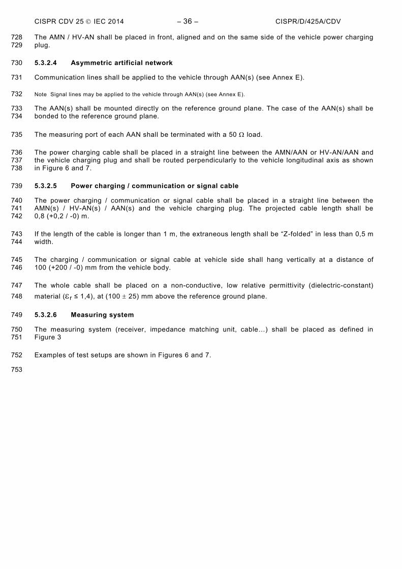
CISPR CDV 25 IEC 2014 – 36 – CISPR/D/425A/CDV The AMN / HV-AN shall be placed in front, aligned and on the same side of the vehicle power charging 728 plug. 729
5.3.2.4 Asymmetric artificial network 730
Communication lines shall be applied to the vehicle through AAN(s) (see Annex E). 731
Note Signal lines may be applied to the vehicle through AAN(s) (see Annex E). 732
The AAN(s) shall be mounted directly on the reference ground plane. The case of the AAN(s) shall be 733 bonded to the reference ground plane. 734
The measuring port of each AAN shall be terminated with a 50 Ω load. 735
The power charging cable shall be placed in a straight line between the AMN/AAN or HV-AN/AAN and 736 the vehicle charging plug and shall be routed perpendicularly to the vehicle longitudinal axis as shown 737 in Figure 6 and 7. 738
5.3.2.5 Power charging / communication or signal cable 739
The power charging / communication or signal cable shall be placed in a straight line between the 740 AMN(s) / HV-AN(s) / AAN(s) and the vehicle charging plug. The projected cable length shall be 741 0,8 (+0,2 / -0) m. 742
If the length of the cable is longer than 1 m, the extraneous length shall be “Z-folded” in less than 0,5 m 743 width. 744
The charging / communication or signal cable at vehicle side shall hang vertically at a distance of 745 100 (+200 / -0) mm from the vehicle body. 746
The whole cable shall be placed on a non-conductive, low relative permittivity (dielectric-constant) 747 material (εr ≤ 1,4), at (100 ± 25) mm above the reference ground plane. 748
5.3.2.6 Measuring system 749
The measuring system (receiver, impedance matching unit, cable…) shall be placed as defined in 750 Figure 3 751
Examples of test setups are shown in Figures 6 and 7. 752
753
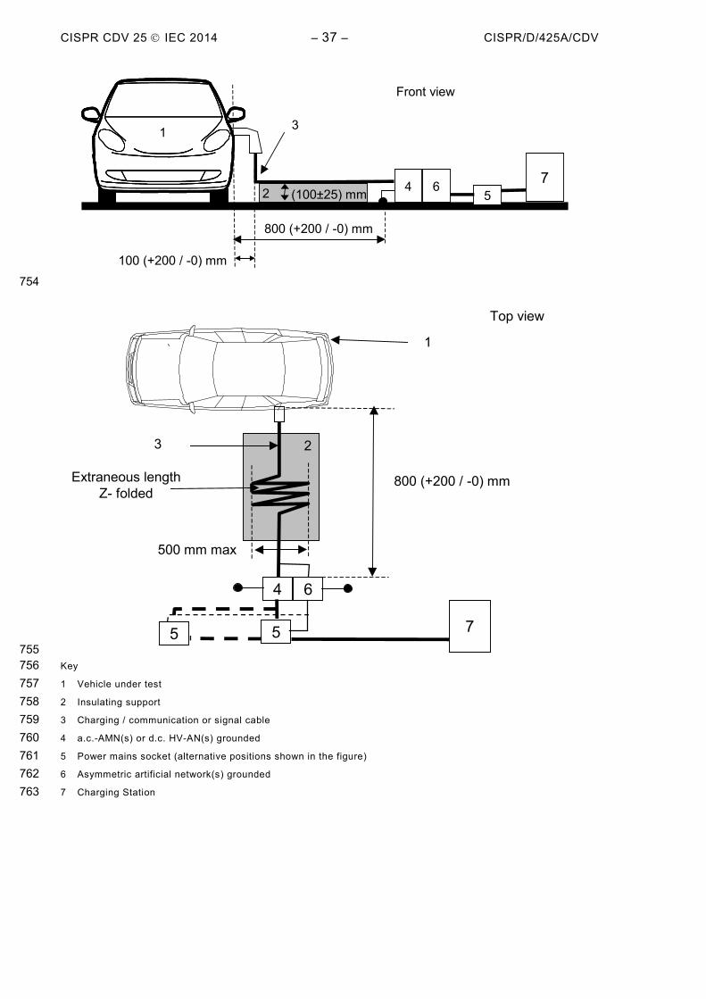
CISPR CDV 25 IEC 2014 – 37 – CISPR/D/425A/CDV
100 (+200 / -0) mm
800 (+200 / -0) mm
5
1 3
2 (100±25) mm 4
Front view
6 7
754
800 (+200 / -0) mmExtraneous lengthZ- folded
4
5
1
23
5
500 mm max
Top view
6
7 755
Key 756 1 Vehicle under test 757 2 Insulating support 758 3 Charging / communication or signal cable 759 4 a.c.-AMN(s) or d.c. HV-AN(s) grounded 760 5 Power mains socket (alternative positions shown in the figure) 761 6 Asymmetric artificial network(s) grounded 762 7 Charging Station 763

CISPR CDV 25 IEC 2014 – 38 – CISPR/D/425A/CDV
Figure 6 – Example of test setup for vehicle with plug located on vehicle side 764 (a.c. or d.c. powered with communication) 765
766

CISPR CDV 25 IEC 2014 – 39 – CISPR/D/425A/CDV
800 (+200 / -0) mm
5
13
2 (100±25) mm 4
Front view
6 7
767
Extraneous lengthZ- folded
1
2
3
500 mm max
Top view
4
5 5
6
7
800 (+200 / -0) mm
100 (+200 / -0) mm
768 Key 769 1 Vehicle under test 770 2 Insulating support 771 3 Charging / communication or signal cable 772 4 a.c. AMN(s) or d.c. HV-AN(s) grounded 773 5 Power mains socket (alternative positions shown in the figure) 774 6 Asymmetric artificial network(s) grounded 775 7 Charging Station 776

CISPR CDV 25 IEC 2014 – 40 – CISPR/D/425A/CDV
Figure 7 – Example of test setup for vehicle with plug located front /rear of vehicle 777 (a.c. or d.c. powered with communication) 778
779 5.4 Examples of limits for vehicle radiated disturbances 780
It is recommended for acceptable radio reception in a vehicle using typical radio receivers, that the 781 disturbance voltage at the end of the antenna cable should not exceed the values shown in Table 4. 782 Where different receivers are used or different coupling models for the propagation of disturbances are 783 valid, the limits may be changed and detailed in the vehicle manufacturer’s own specification. 784
785 786

CISPR CDV 25 IEC 2014 – 41 – CISPR/D/425A/CDV
Table 4 – Example for limits of disturbance – Complete vehicle 787
Service / Band a Frequency
MHz Terminal disturbance voltage at receiver antenna terminal in dB (mV)
Peak Quasi-peak Average
BROADCAST
LW b 0,15 - 0,30 26 13 6
MW b 0,53 - 1,8 20 7 0
SW b 5,9 - 6,2 20 7 0
FM b 76 - 108 26 13 6
TV Band I c 41 - 88 16 - 6
TV Band III c 174 - 230 16 - 6
DAB III 171 - 245 10 - 0
TV Band IV/V c 468 - 944 16 - 6
DTTV 470 - 770 20 d - 10 d DAB L band 1 447 – 1 494 10 - 0 SDARS 2 320 – 2 345 16 - 6
MOBILE SERVICES
CB b 26 - 28 20 7 0
VHF b 30 - 54 20 7 0
VHF b 68 - 87 20 7 0
VHF b 142 -175 20 7 0
Analogue UHF b 380 - 512 20 7 0
RKE f 300 - 330 20 - 6
RKE f 420 - 450 20 - 6
Analogue UHF b 820 - 960 20 7 0
GSM 800 860 - 895 26 - 6
EGSM/GSM 900 925 - 960 26 - 6
GPS L1 civil e,g 1 567 – 1 583 - - 0
GLONASS L1 e,h 1 591 – 1 613 - - 0
GSM 1800 (PCN) 1 803 – 1 882 26 - 6 GSM 1900 1 850 – 1 990 26 - 6 3G / IMT 2000 1 900 – 1 992 26 - 6 3G / IMT 2000 2 010 – 2 025 26 - 6 3G / IMT 2000 2 108 – 2 172 26 - 6 Bluetooth/802.11 2 400 – 2 500 26 - 6

CISPR CDV 25 IEC 2014 – 42 – CISPR/D/425A/CDV a LW: Long wave, MW: Medium wave, SW: Short wave (amplitude modulation, AM) VHF: Very high frequency, UHF: Ultra high frequency (frequency modulation, FM) DAB: Digital audio broadcasting, TV: Television, DTTV: Digital Terrestrial Television RKE: Remote keyless entry, GPS: Global positioning system, GSM: Global system mobile 3G: Third generation b In this analogue service the peak and quasi-peak limits can be relaxed by 6 dB for short duration disturbances
(e.g. short duration PK (or QPK) limit = PK (or QPK) limit + 6 dB) c Analogue TV only d This limit is less stringent than the analogue limit and should only be applied where analogue TV is no longer in
use e The bandwidth and frequency steps to be used for the GPS and GLONASS L1 civil band are respectively 9 kHz
and 5 kHz rather than the bandwidth and frequency steps defined in Table 1 and Table 2 for services above 30 MHz.
f RKE limits are defined over a large frequency band. Any modification of the average limit around the operating frequency due to sensitivity of RKE systems should be defined in the test plan.
g The values given in the table apply for the 1 574,42 MHz to 1 576,42 MHz frequency range. The limits for the whole GPS L1 frequency range are given in Figure 8a.
h The values given in the table apply for the 1 598,065 MHz to 1 606,5 MHz frequency range. The limits for the whole GLONASS L1 frequency range are given in Figure 8b.
NOTE 1 Stereo signals may be more susceptible to disturbance than monaural signals in the FM broadcast band. This phenomenon has been factored into the FM (76 MHz to 108 MHz) limits.
NOTE 2 All values listed in this table are valid for the bandwidths in Tables 1 and 2. If measurements have to be performed with different bandwidths than those specified in Tables 1 and 2 because of ambient noise requirements, then applicable limits should be defined in the test plan and the applied limits and bandwidths should be documented in the test report.
788
-10
0
10
20
30
40
50
1567
,42
1568
,42
1569
,42
1570
,42
1571
,42
1572
,42
1573
,42
1574
,42
1575
,42
1576
,42
1577
,42
1578
,42
1579
,42
1580
,42
1581
,42
1582
,42
1583
,42
Leve
l in
dB(µ
V)
frequency in MHz 789
Figure 8a – Average limit for radiated disturbances from vehicles GPS band 790 1 567,42 to 1 583,42 MHz 791

CISPR CDV 25 IEC 2014 – 43 – CISPR/D/425A/CDV
-10
0
10
20
30
40
50
1591
,065
1592
,065
1593
,065
1594
,065
1595
,065
1596
,065
1597
,065
1598
,065
1606
,500
1607
,500
1608
,500
1609
,500
1610
,500
1611
,500
1612
,500
1613
,500
Leve
l in
dB(µ
V)
frequency in MHz 792
Figure 8b – Average limit for radiated disturbance from vehicles GLONASS band 793 1 591,065 to 1 613,5 MHz 794
795
NOTE - If an active antenna is used, the noise floor may increase. The additional noise floor depends on the type of antenna 796 and must be subtracted from the measured value to determine the real value of the disturbance using the following formula (all 797 terms in μV): 798
22noiseAntennaMeasuredeDisturbancreal UUU −= (2) 799
A relaxation of the limit because of the active antenna noise floor does not guarantee compliance. Subsequent changes to the 800 active antenna design may result in non-compliance. This topic remains under study. Annex D describes a method to determine 801 the noise floor of an active antenna. 802
803
804

CISPR CDV 25 IEC 2014 – 44 – CISPR/D/425A/CDV
6 Measurement of components and modules 805
6.1 General 806
For LV components test methods and requirements are defined in this clause. 807
For LV/HV components additional test methods and limits are defined in Annex I. 808
For LV/HV components: 809
– Conducted emission (voltage method) on LV lines shall be performed according to setup defined 810 in clause I.3 and requirement in 6.2.3 811
– Conducted emission (voltage method) on HV lines shall be performed according to setup defined 812 in clause I.3 and requirement in I.3.3 813
6.2 Test equipment 814
6.2.1 Reference ground plane 815
The reference ground plane shall be defined as the top metallic surface of the test bench/table. 816
The reference ground plane shall be made of 0,5 mm thick (minimum) copper, brass, bronze or 817 galvanized steel. 818
The minimum size of the reference ground plane for conducted emissions (voltage method) shall be 819 1 000 mm x 400 mm. 820
The minimum size of the reference ground plane for conducted emissions (current probe method) shall 821 be 2 500 mm x 400 mm. 822
The minimum width of the reference ground plane for radiated emissions shall be 1 000 mm. The 823 minimum length of the reference ground plane for radiated emissions shall be 2 000 mm, or underneath 824 the entire equipment plus 200 mm, whichever is larger. 825
The height of the reference ground plane (test bench) shall be (900 ± 100) mm above the floor. 826
The distance from the edge of the ground strap to the edge of the next strap shall not be greater than 827 300 mm. The maximum length to width ratio for the ground straps shall be 7:1. 828
Note 1 Because of resonances of the reference ground plane the location, width and length of the bond straps may influence 829 the measurement results. A sufficient number of low inductive bond straps are necessary to ensure a low impedance 830 connection to the shielded room. 831
6.2.2 Power supply and AN 832
For the tests defined in 6.3, 6.4, 6.5, 6.6 and 6.7, each positive EUT power supply lead shall be 833 connected to the power supply through an artificial network. For the TEM cell emissions tests of 6.6, an 834 AN with a coaxial connector will facilitate connection to the TEM cell EUT power connector. The AN 835 shall have a nominal 5 mH inductance. The impedance characteristics and a suggested schematic are 836 shown in Annex E. 837

CISPR CDV 25 IEC 2014 – 45 – CISPR/D/425A/CDV Power supply is assumed to be negative ground. If the EUT utilizes a positive ground then the test 838 setups shown in the figures need to be adapted accordingly. Depending on the intended EUT 839 installation in the vehicle: 840
– EUT remotely grounded (vehicle power return line longer than 200 mm): two artificial networks 841 are required, one for the positive supply line and one for the power return line. 842
– EUT locally grounded (vehicle power return line 200 mm or shorter): one artificial network is 843 required, for the positive supply. 844
The AN(s) shall be mounted directly on the reference ground plane. The case(s) of the AN(s) shall be 845 bonded to the reference ground plane. The d.c. resistance between the ground of the AN measurement 846 port and the ground plane shall not exceed 2,5 mΩ 847
The power supply return shall be connected to the reference ground plane (between the power supply 848 and the AN(s)). 849
The measuring port of the AN not connected to the measuring instrument shall be terminated with a 50 Ω load. 850
6.2.3 Load Simulator 851
The load simulator includes sensors and actuators, and terminates the test harness connected to the 852 EUT. 853
To ensure sufficient reproducibility the same termination must be used for each measurement either by 854 using special termination equipment (e.g. artificial networks, filters) – located at the RF boundary – or 855 by using the same load simulator. 856
6.2.4 Signal/control line filters 857
In the TEM cell test method using the coaxial connectors for EUT leads each lead shall pass through a 858 filter which has impedance characteristics similar to that of the AN defined above. 859
The attenuation of the filters shall be specified for the whole frequency range of the intended 860 component/module test (see 6.3 to 6.7) according to the requirements shown in Figure 9. The minimum 861 attenuation shall be more than 40 dB from 30 MHz up to the upper cut-off frequency (fc), which depends 862 on the intended test method. Figure 9 shows e.g. an upper cut-off frequency (fc) of the chosen test 863 method of 400 MHz. 864
NOTE Other low pass RF filter configurations may be used if the filter characteristics are not applicable to special wanted 865 signals of the EUT's inputs or outputs (e.g. high speed network data interfaces). The filters shall be specified in the test plan. 866
867

CISPR CDV 25 IEC 2014 – 46 – CISPR/D/425A/CDV
0
10
20
30
40
50
1 10 100 1000Frequency MHz
Atte
nuat
ion
dB
868
Figure 9 – Example for the required minimum attenuation 869 of the Signal / Control line filters 870
The attenuation of such a filter can be determined by a two-port network analyser measurement (-s21). 871 The input and output impedance of the network analyzer shall be 50 Ω. 872
The test setup is shown in Figure 10. 873
Note Equivalent methods for measuring in a 50 Ω system such as a measuring receiver or equivalent equipment with built-in 874 tracking generator can also be used for the measurement since only the magnitude of the attenuation is to be measured. 875
876
network analyzer
signal/control
linefilter
877 878
Figure 10 – Setup for measurement of the filter attenuation 879
6.3 Conducted emissions from components/modules – Voltage method 880
6.3.1 General 881
Voltage measurements are able to characterize the emissions on single leads only. The test method is 882 not usable to characterize the radiated emission transmitted e.g. by different antenna structures on the 883 printed board of electronic components or to characterize the efficiency of shielding. Therefore, voltage 884 measurements are not able to characterize the complete EUT emission. At lower frequencies (e.g. in 885 the AM-bands) voltage measurements usually ensure more dynamic range than radiated measurements. 886
(fc)

CISPR CDV 25 IEC 2014 – 47 – CISPR/D/425A/CDV 6.3.2 Reference ground plane arrangement 887
6.3.2.1 Test setup 888
6.3.2.1.1 Location of the EUT 889
The EUT shall be placed on a non-conductive, low relative permittivity material (εr ≤ 1,4), at (50 ± 5) mm 890 above the reference ground plane. 891
The case of the EUT shall not be grounded to the reference ground plane unless it is intended to 892 simulate the actual vehicle configuration. 893
All sides of the EUT shall be at least 100 mm from the edge of the reference ground plane. In the case 894 of a grounded EUT, the ground connection point shall also have a minimum distance of 100 mm from 895 the edge of the reference ground plane. 896
6.3.2.1.2 Location of the test harness 897
The power supply line(s) between the connector of the AN(s) and the connector(s) of the EUT ( lp) shall 898 have a standard length of ( )200
0200 + mm. 899
The harness shall be placed in a straight line on a non-conductive, low relative permittivity material 900 (εr ≤ 1,4), at (50 ± 5) mm above the reference ground plane. 901
To minimize the coupling between power and input/output leads, the space between those lead types 902 shall be maximized (≥ 200 mm from or perpendicular to the power supply lines connecting the AN(s) 903 and the EUT). 904
The total length of the test harness (excluding power lines) shall not exceed 2 m. The wiring type is 905 defined by the actual system application and requirement. 906
All leads and cables shall be located at a minimum distance of 100 mm from the edge of the reference 907 ground plane. 908
6.3.2.1.3 Location of the load simulator 909
Preferably, the load simulator shall be placed directly on the reference ground plane. If the load 910 simulator has a metallic case, this case shall be bonded to the reference ground plane. 911
Note Alternatively, the load simulator may be located adjacent to the reference ground plane (with the case of the load 912 simulator bonded to the reference ground plane) or outside of the test chamber, provided the test harness from the EUT passes 913 through an RF boundary bonded to the reference ground plane. 914
When the load simulator is located on the reference ground plane, the d.c. power supply lines of the 915 load simulator shall be connected directly to the power supply and not through the AN(s). 916
6.3.2.2 Test procedure 917
The general arrangement of the disturbance source (EUT), connecting harnesses, etc. represents a 918 standardised test condition. Any deviations from the standard test harness length etc. shall be agreed 919 upon prior to testing and recorded in the test report. 920

CISPR CDV 25 IEC 2014 – 48 – CISPR/D/425A/CDV The EUT shall be made to operate under typical loading and other conditions as in the vehicle such that 921 the maximum emission state occurs. These operating conditions must be clearly defined in the test plan 922 to ensure supplier and customer are performing identical tests. 923
The conducted emissions on power lines are measured successively on positive power supply and 924 power return by connecting the measuring instrument on the measuring port of the related AN, the 925 measuring port of the AN in the other supply lines being terminated with a 50 Ω load. 926
For voltage measurements the following apply: 927
– For EUT remotely grounded (vehicle power return line longer than 200 mm), the voltage meas-928 urements shall be made on each lead (supply and return) relative to the reference ground plane 929 (see Figure 11). 930
– For EUT locally grounded (vehicle power return line 200 mm or shorter), voltage measurements 931 on power supply leads shall be made relative to the reference ground plane (see Figure 12). 932
– Generators/alternators shall be loaded with a battery and parallel resistor combination, and 933 connected to the artificial network in the manner shown in Figure 13. The load current, operating 934 speed, harness length and other conditions shall be defined in the test plan. 935
– For the tests of ignition systems refer to Figure 14. 936
Note For EUT's with multiple positive power supply connections and/or multiple power return connections, the measurements 937 (on power supply and on power return) may be performed with all power supply connections tied together at the AN and all 938 power return connections tied together at the other AN. The details of the AN connection should be defined in the test plan. 939
940 941

CISPR CDV 25 IEC 2014 – 49 – CISPR/D/425A/CDV
Dimensions in millimetres – not to scale 942 943
5
7
6 50 ±
5
Side view
23
1
Top view
12
2
4
9
12
3
100 min
8
6
6
7
11
200+2000
5
10
13
944 945
946 Key
1 Power supply (may be placed on the reference ground plane)
2 Artificial network
3 EUT (housing grounded if required in test plan)
4 Load simulator (metallic casing grounded if required in test plan)
5 Reference ground plane
6 Power supply lines
7 Low relative permittivity support (εr≤ 1,4)
8 High-quality coaxial cable e.g. double-shielded (50 Ω)
9 Measuring instrument 10 Shielded enclosure
11 50 Ω load
12 Bulkhead connector
13 Test harness (excluding power lines)
Note The EUT housing ground lead, when required in the test plan, should not be longer than 150 mm.
Figure 11 – Conducted emissions – Example of test setup for EUT with power return line 947 remotely grounded. 948
949

CISPR CDV 25 IEC 2014 – 50 – CISPR/D/425A/CDV
Dimensions in millimetres – not to scale 950 951
5
7
6 50 ±
5
Side view
23
1
Top view
12
4
9
12
3
100 min
8
6
7
200+2000
5
10
13
952 953
954 Key
1 Power supply (may be placed on the reference ground plane)
2 Artificial network
3 EUT (housing grounded if required in test plan)
4 Load simulator (metallic casing grounded if required in test plan)
5 Reference ground plane
6 Power supply line
7 Low relative permittivity support (εr ≤ 1,4)
8 High-quality coaxial cable e.g. double-shielded (50 Ω)
9 Measuring instrument
10 Shielded enclosure
12 Bulkhead connector
13 Test harness (excluding power lines)
Note The EUT housing ground lead, when required in the test plan, should not be longer than 150 mm.
955 Figure 12 – Conducted emissions – Example of test setup for EUT with power return line locally 956
grounded 957
958

CISPR CDV 25 IEC 2014 – 51 – CISPR/D/425A/CDV 959
Dimensions in millimetres – not to scale 960
5
6
Side view
231
Top view
12
4
9
12
3
100 min
8
6
200+2000
5
10
14
15
14
15
16
16
17
13
961 962
Key
1 Battery (may be placed on the reference ground plane)
2 Artificial network
3 EUT
4 Load simulator (metallic casing grounded if required in test plan)
5 Reference ground plane
6 Power supply lines
8 High-quality coaxial cable e.g. double-shielded (50 Ω)
9 Measuring instrument
10 Shielded enclosure
11 50 Ω load
12 Bulkhead connector
13 Test harness (excluding power lines)
14 Motor (Air/Low Emissions)
15 Non-conductive belt/coupler
16 Load resistor
17 Indicator lamp/control resistor (if applicable)
Note The EUT housing ground lead, when required in the test plan, should not be longer than 150 mm.
963

CISPR CDV 25 IEC 2014 – 52 – CISPR/D/425A/CDV
Figure 13 – Conducted emissions – Example of test setup for alternators and generators 964
965

CISPR CDV 25 IEC 2014 – 53 – CISPR/D/425A/CDV
Dimensions in millimetres – not to scale 966
967
968 Key
1 Power supply (may be placed on the reference ground plane)
2 Artificial network
3 Pencil coil
4 ECU simulator (metallic casing grounded if required in test plan)
5 Reference ground plane
7 Low relative permittivity support (εr ≤ 1,4)
8 High-quality coaxial cable e.g. double-shielded (50 Ω)
9 Measuring instrument
10 Shielded enclosure
11 50 Ω load
12 Bulkhead connector
13 Optical fibres
14 Fiber optic feed through
15 Optical fibre converter
16 1 000 µF capacitor
17 Engine simulator
18 Battery
19 Signal line
Note The pencil coil housing ground lead, when required in the test plan, should not be longer than 150 mm.
5
7
-
1
+
+-
18
15
4
2
2
-
17
19
+16
9
8
200
3
10
13
12
± 10
14
100
min
11

CISPR CDV 25 IEC 2014 – 54 – CISPR/D/425A/CDV
969 Figure 14 – Conducted emissions – Example of test setup for ignition system components 970
971

CISPR CDV 25 IEC 2014 – 55 – CISPR/D/425A/CDV 6.3.3 Limits for conducted disturbances from components/modules – Voltage method 972
The level class to be used (as a function of the frequency band) shall be agreed upon between the 973 vehicle manufacturer and the component supplier. 974
Note 1 The method to be used for characterisation of the Voltage Division Factor of the AN, sometimes referred to as insertion 975 loss, is given in Annex A.8 of CISPR 16-1-2. 976
Note 2 It is recommended for acceptable radio reception in a vehicle that the conducted noise should not exceed the values 977 shown in Table 5, peak and average or quasi-peak and average, respectively. Since the mounting location, vehicle body 978 construction and harness design can affect the coupling of radio disturbances to the on-board radio, multiple limit levels are 979 defined. 980
981

CISPR CDV 25 IEC 2014 – 56 – CISPR/D/425A/CDV
Table 5 – Examples of limits for conducted disturbances – 982 Voltage Method 983
Service / Band Frequency
MHz
Levels in dB(µV)
Class 5 Class 4 Class 3 Class 2 Class 1
Pea
k
Qua
sipe
ak
Ave
rage
Pea
k
Qua
sipe
ak
Ave
rage
Pea
k
Qua
sipe
ak
Ave
rage
Pea
k
Qua
sipe
ak
Ave
rage
Pea
k
Qua
sipe
ak
Ave
rage
BROADCAST LW 0,15 – 0,30 70 57 50 80 67 60 90 77 70 100 87 80 110 97 90 MW 0,53 – 1,8 54 41 34 62 49 42 70 57 50 78 65 58 86 73 66 SW 5,9 – 6,2 53 40 33 59 46 39 65 52 45 71 58 51 77 64 57 FM 76 – 108 38 25 18 44 31 24 50 37 30 56 43 36 62 49 42 TV Band I 41 – 88 34 - 24 40 - 30 46 - 36 52 - 42 58 - 48 TV Band III 174 – 230
Conducted emission – Voltage method Not Applicable
DAB III 171 – 245 TV Band IV 468 – 944 DTTV 470 – 770 DAB L Band 1447 – 1494 SDARS 2320 – 2345
MOBILE SERVICES CB 26 – 28 44 31 24 50 37 30 56 43 36 62 49 42 68 55 48 VHF 30 – 54 44 31 24 50 37 30 56 43 36 62 49 42 68 55 48 VHF 68 – 87 38 25 18 44 31 24 50 37 30 56 43 36 62 49 42 VHF 142 – 175
Conducted emission – Voltage method Not Applicable
Analogue UHF 380 – 512 RKE 300 – 330 RKE 420 – 450 Analogue UHF 820 – 960 GSM 800 860 – 895 EGSM/GSM 900 925 – 960 GPS L1 civil 1567 – 1583 GLONASS L1 1 591 – 1 613 GSM 1800 (PCN) 1803 – 1882 GSM 1900 1850 – 1990 3G / IMT 2000 1900 – 1992 3G / IMT 2000 2010 – 2025 3G / IMT 2000 2180 – 2172 Bluetooth/802.11 2400 – 2500 Note 1 All values listed in this table are valid for the bandwidths in Tables 1 and 2. If measurements have to be performed with different bandwidths than those specified in Tables 1 and 2 because of noise floor requirements, then applicable limits should be defined in the test plan. Note 2 Where multiple bands use the same limits the user must select the appropriate bands over which to test. – When the test plan includes bands that overlap the test plan shall define the applicable limit. Note 3 Although the limits for Peak, Quasi-Peak and Average detectors are shown, measurements with all three detectors are not required. See Figure 1.
984 985

CISPR CDV 25 IEC 2014 – 57 – CISPR/D/425A/CDV 6.4 Conducted emissions from components/modules – current probe method 986
6.4.1 Test setup 987
6.4.1.1 Location of the EUT 988
The EUT shall be placed on a non-conductive, low relative permittivity material (εr ≤ 1,4), at (50 ± 5) mm 989 above the reference ground plane. 990
The case of the EUT shall not be grounded to the reference ground plane unless it is intended to 991 simulate the actual vehicle configuration. 992
The EUT shall be at least 100 mm from the edge of the reference ground plane and at least 500 mm 993 from the chamber wall. The test plan shall simulate the actual vehicle configuration and shall specify: 994 remote versus local grounding, the use of an insulating spacer, and the electrical connection of the EUT 995 case to the reference ground plane. 996
The measuring equipment shall be as shown in Figure 15. 997
6.4.1.2 Location of the test harness 998
The test harness shall be ( )3000700 1 + mm long (or as agreed upon in the test plan), and shall be placed 999
on a non-conductive, low relative permittivity material (εr ≤ 1,4), positioned (50 ± 5) mm above the 1000 reference ground plane. The test harness wires shall be nominally parallel and adjacent unless 1001 otherwise defined in the test plan. 1002
6.4.2 Test procedure 1003
The probe (see CISPR 16-1-2) shall be mounted around the complete harness (including all wires). If 1004 the EUT has multiple connectors on the unit resulting in multiple wire bundles, the test plan shall define 1005 which wires shall be included in the probe for measurement. In the absence of any definition, 1006 measurements shall be made for each bundle (connector) independently and for all wires together. 1007
If the EUT wiring has too many wires to be accommodated in the measurement probe, the test plan may 1008 define the wires to be measured and this shall be included in the test report. 1009
Measure the emissions with the probe positioned 50 mm and 750 mm from the EUT. 1010
In most cases, the position of maximum emission will be as close to the EUT connector as possible. 1011 Where the EUT is equipped with a metal shell connector, the probe shall be clamped to the cable 1012 immediately adjacent to the connector shell, but not around the connector shell itself. The EUT shall be 1013 at least 100 mm from the edge of the reference ground plane and at least 500 mm from the chamber 1014 wall. The test plan shall simulate the actual vehicle configuration and shall specify remote versus local 1015 grounding, the use of an insulating spacer and the electrical connection of the EUT case to the 1016 reference ground plane. 1017
Note Some additional measurements may be defined in the test plan with only the positive supply wire in the probe and/or only 1018 the negative supply wire in the probe. For these test configurations limits are to be defined in the test plan. 1019
1020
1021

CISPR CDV 25 IEC 2014 – 58 – CISPR/D/425A/CDV
1022
1023 Dimensions in millimetres – not to scale 1024
1025
Key
1 Power supply
2 Artificial network
3 EUT (connected to ground if specified in the test plan)
4 Load simulator (metallic casing grounded if required in test plan)
5 Reference ground plane
6 Wiring harness
7 Low relative permittivity support (εr ≤ 1,4)
8 High-quality coaxial cable e.g. double-shielded (50 Ω)
9 Measuring instrument
10 Shielded enclosure
11 Fiber optic feed through
12 Bulkhead connector
13 Optical fibers
14 Current probe (represented at 2 positions)
15 Stimulation and monitoring system
d The distance from the EUT to the closest probe position
1026
200 min.
+ -
500 min
100 min
1 5
13
7
10
6 14 7
3 4
±
± 50 5
900 100
1700 +300 / - 0 2500 min
3 d
14 7
4
15 9
2 2
8
12 11
14
14
200 min.
+ -
500 min
100 min
1 5
13
7
10
6 14 7
3 4
±
± 50 5
900 100
1700 +300 / - 0 2500 min
3 d
14 7
4
15 9
2 2
8
12
14
14

CISPR CDV 25 IEC 2014 – 59 – CISPR/D/425A/CDV
Figure 15– Conducted emissions – Example of test setup 1027 for current probe measurements 1028
1029

CISPR CDV 25 IEC 2014 – 60 – CISPR/D/425A/CDV 6.4.3 Limits for conducted disturbances from components/modules – Current probe method 1030
The level class to be used (as a function of the frequency band) shall be agreed upon between the 1031 vehicle manufacturer and the component supplier. 1032
Note It is recommended for acceptable radio reception in a vehicle that the conducted noise should not exceed the values 1033 shown in Table 6, peak and average or quasi-peak and average limits, respectively. Since the mounting location, vehicle body 1034 construction and harness design can affect the coupling of radio disturbances to the on-board radio, multiple limit levels are 1035 defined. 1036
Table 6 – Examples of limits for conducted disturbances - control/signal lines – Current probe 1037 method 1038
Service / Band Frequency
MHz
Levels in dB(µA)
Class 5 Class 4 Class 3 Class 2 Class 1
Pea
k
Qua
sipe
ak
Ave
rage
Pea
k
Qua
sipe
ak
Ave
rage
Pea
k
Qua
sipe
ak
Ave
rage
Pea
k
Qua
sipe
ak
Ave
rage
Pea
k
Qua
sipe
ak
Ave
rage
BROADCAST LW 0,15 – 0,30 50 37 30 60 47 40 70 57 50 80 67 60 90 77 70 MW 0,53 – 1,8 26 13 6 34 21 14 42 29 22 50 37 30 58 45 38 SW 5,9 – 6,2 19 6 -1 25 12 5 31 18 11 37 24 17 43 30 23 FM 76 – 108 4 -9 -16 10 -3 -10 16 3 -4 22 9 2 28 15 8 TV Band I 41 – 88 0 - -10 6 - -4 12 - 2 18 - 8 24 - 14 DAB III 171 – 245 -2 - -12 4 - -6 10 - 0 16 - 6 22 - 12 TV Band III 174 – 230
Conducted emission – control/signal lines
Not Applicable
TV Band IV 468 – 944 DTTV 470 – 770 DAB L Band 1447 – 1494 SDARS 2320 – 2345
MOBILE SERVICES CB 26 – 28 10 -3 -10 16 3 -4 22 9 2 28 15 8 34 21 14 VHF 30 – 54 10 -3 -10 16 3 -4 22 9 2 28 15 8 34 21 14 VHF 68 – 87 4 -9 -16 10 1 -10 16 7 -4 22 13 2 28 15 8 VHF 142-175 4 -9 -16 10 1 -10 16 7 -4 22 13 2 28 15 8 Analogue UHF 380 – 512
Conducted emission – control/signal lines
Not Applicable
RKE 300 – 330 RKE 420 – 450 Analogue UHF 820 – 960 GSM 800 860 – 895 EGSM/GSM 900 925 – 960 GPS L1 civil 1567 – 1583 GLONASS L1 1 591 – 1 613 GSM 1800 (PCN) 1803 – 1882 GSM 1900 1850 – 1990 3G / IMT 2000 1900 – 1992 3G / IMT 2000 2010 – 2025 3G / IMT 2000 2180 – 2172 Bluetooth/802.11 2400 – 2500 Note 1 All values listed in this table are valid for the bandwidths in Tables 1 and 2. If measurements have to be performed with different bandwidths than those specified in Tables 1 and 2 because of noise floor requirements, then applicable limits should be defined in the test plan. Note 2 Where multiple bands use the same limits the user must select the appropriate bands over which to test. – When the test plan includes bands that overlap the test plan shall define the applicable limit.

CISPR CDV 25 IEC 2014 – 61 – CISPR/D/425A/CDV
Note 3 Although the limits for Peak, Quasi-Peak and Average detectors are shown, measurements with all three detectors are not required. See Figure 1.
1039 1040
6.5 Radiated emissions from components/modules - ALSE method 1041
6.5.1 General 1042
Measurements of radiated field strength shall be made in an ALSE to eliminate the high levels of 1043 extraneous disturbance from electrical equipment and broadcasting stations. 1044
Note 1 Conducted emissions will contribute to the radiated emissions measurements because of radiation from the wiring in 1045 the test setup. Therefore, it is advisable to establish conformance with the conducted emissions requirements before 1046 performing the radiated emissions test. 1047
Note 2 Disturbance to the vehicle on-board receiver can be caused by direct radiation from one or more leads in the vehicle 1048 wiring harness. This coupling mode to the vehicle receiver affects both the type of testing and the means of reducing the 1049 disturbance at the source. 1050
Note 3 Vehicle components which are not effectively grounded to the vehicle by short ground leads, or which have several 1051 harness leads carrying the disturbance voltage, will have radiated emissions that do not correlate well with its conducted 1052 emissions. This has been shown to give better correlation with the complete vehicle test for components installed in this way. 1053
Examples of component installations for which this test is applicable include, but are not limited to: 1054
– electronic control systems containing microprocessors; 1055 – two speed wiper motors with negative supply switching; 1056 – suspension control systems with strut-mounted actuator motors; 1057 – engine cooling and heater blower motors mounted in plastic or other insulated housings. 1058
6.5.2 Test setup 1059
For radiated emissions measurements, the arrangement of the EUT, test harness, load simulator and 1060 measuring equipment shall be equivalent to the examples shown in Figures 17 to 20. 1061
6.5.2.1 Antenna systems 1062
Measurements shall be made using linearly polarised electric field antennas that have a nominal 50 Ω 1063 output impedance. 1064
Note 1 To improve consistency of results between laboratories, the following antennas are recommended: 1065 1066 a) 0,15 MHz to 30 MHz 1 m vertical monopole (where this is not 50 Ω, a suitable antenna matching 1067 unit shall be used); 1068 1069 b) 30 MHz to 300 MHz a biconical antenna; 1070 1071 c) 200 MHz to 1 000 MHz a log-periodic antenna; 1072 1073 d) 1 000 MHz to 2 500 MHz a horn or log periodic antenna. 1074
The method to be used for characterization of the vertical monopole (rod) antenna is given in CISPR 16-1075 1-4. 1076
Note 2 Use the 1 m method in SAE ARP 958.1 Rev D February 2003 for determining biconical, log periodic and horn antenna 1077 factors. 1078

CISPR CDV 25 IEC 2014 – 62 – CISPR/D/425A/CDV Note 3 Biconical antennas usually have a SWR of up to 10:1 in the frequency range of 30 MHz to 80 MHz. Therefore an 1079 additional measurement error may occur when the receiver input impedance differs from 50 Ω. The use of an attenuator (3 dB 1080 minimum) at the receiver's input or the input of an additional preamplifier (if possible) will keep this additional error low. 1081
1082
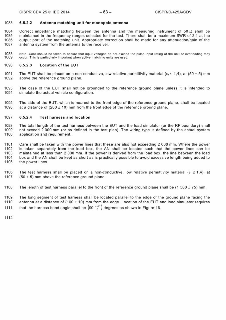
CISPR CDV 25 IEC 2014 – 63 – CISPR/D/425A/CDV 6.5.2.2 Antenna matching unit for monopole antenna 1083
Correct impedance matching between the antenna and the measuring instrument of 50 Ω shall be 1084 maintained in the frequency ranges selected for the test. There shall be a maximum SWR of 2:1 at the 1085 output port of the matching unit. Appropriate correction shall be made for any attenuation/gain of the 1086 antenna system from the antenna to the receiver. 1087
Note Care should be taken to ensure that input voltages do not exceed the pulse input rating of the unit or overloading may 1088 occur. This is particularly important when active matching units are used. 1089
6.5.2.3 Location of the EUT 1090
The EUT shall be placed on a non-conductive, low relative permittivity material (εr ≤ 1,4), at (50 ± 5) mm 1091 above the reference ground plane. 1092
The case of the EUT shall not be grounded to the reference ground plane unless it is intended to 1093 simulate the actual vehicle configuration. 1094
The side of the EUT, which is nearest to the front edge of the reference ground plane, shall be located 1095 at a distance of (200 ± 10) mm from the front edge of the reference ground plane. 1096
6.5.2.4 Test harness and location 1097
The total length of the test harness between the EUT and the load simulator (or the RF boundary) shall 1098 not exceed 2 000 mm (or as defined in the test plan). The wiring type is defined by the actual system 1099 application and requirement. 1100
Care shall be taken with the power lines that these are also not exceeding 2 000 mm. Where the power 1101 is taken separately from the load box, the AN shall be located such that the power lines can be 1102 maintained at less than 2 000 mm. If the power is derived from the load box, the line between the load 1103 box and the AN shall be kept as short as is practically possible to avoid excessive length being added to 1104 the power lines. 1105
The test harness shall be placed on a non-conductive, low relative permittivity material (εr ≤ 1,4), at 1106 (50 ± 5) mm above the reference ground plane. 1107
The length of test harness parallel to the front of the reference ground plane shall be (1 500 ± 75) mm. 1108
The long segment of test harness shall be located parallel to the edge of the ground plane facing the 1109 antenna at a distance of (100 ± 10) mm from the edge. Location of the EUT and load simulator requires 1110 that the harness bend angle shall be ( )5
090 4+ degrees as shown in Figure 16. 1111
1112
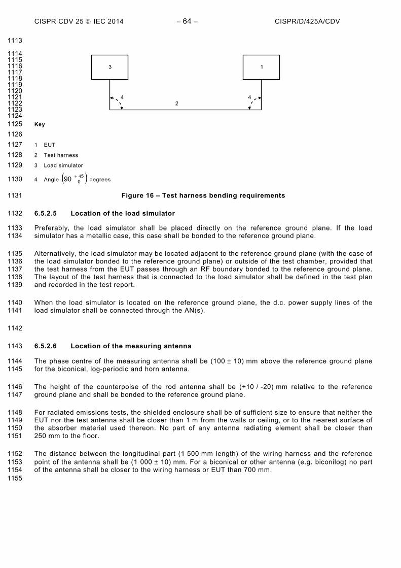
CISPR CDV 25 IEC 2014 – 64 – CISPR/D/425A/CDV 1113
1114 1115 1116 1117 1118 1119 1120 1121 1122 1123 1124 Key 1125 1126 1 EUT 1127 2 Test harness 1128 3 Load simulator 1129
4 Angle ( )5090 4+
degrees 1130
Figure 16 – Test harness bending requirements 1131
6.5.2.5 Location of the load simulator 1132
Preferably, the load simulator shall be placed directly on the reference ground plane. If the load 1133 simulator has a metallic case, this case shall be bonded to the reference ground plane. 1134
Alternatively, the load simulator may be located adjacent to the reference ground plane (with the case of 1135 the load simulator bonded to the reference ground plane) or outside of the test chamber, provided that 1136 the test harness from the EUT passes through an RF boundary bonded to the reference ground plane. 1137 The layout of the test harness that is connected to the load simulator shall be defined in the test plan 1138 and recorded in the test report. 1139
When the load simulator is located on the reference ground plane, the d.c. power supply lines of the 1140 load simulator shall be connected through the AN(s). 1141
1142
6.5.2.6 Location of the measuring antenna 1143
The phase centre of the measuring antenna shall be (100 ± 10) mm above the reference ground plane 1144 for the biconical, log-periodic and horn antenna. 1145
The height of the counterpoise of the rod antenna shall be (+10 / -20) mm relative to the reference 1146 ground plane and shall be bonded to the reference ground plane. 1147
For radiated emissions tests, the shielded enclosure shall be of sufficient size to ensure that neither the 1148 EUT nor the test antenna shall be closer than 1 m from the walls or ceiling, or to the nearest surface of 1149 the absorber material used thereon. No part of any antenna radiating element shall be closer than 1150 250 mm to the floor. 1151
The distance between the longitudinal part (1 500 mm length) of the wiring harness and the reference 1152 point of the antenna shall be (1 000 ± 10) mm. For a biconical or other antenna (e.g. biconilog) no part 1153 of the antenna shall be closer to the wiring harness or EUT than 700 mm. 1154
1155
2 4 4
1 3

CISPR CDV 25 IEC 2014 – 65 – CISPR/D/425A/CDV The reference point of the antenna is defined as: 1156
– the vertical monopole element for rod antennas, 1157 – the phase centre (mid-point) for biconical antennas, 1158 – the tip for antennas with log-periodic elements (including biconilog antennas), 1159 – the front aperture for horn antennas. 1160
Each antenna (excluding the rod antenna) shall be calibrated for this reference point for a 1 000 mm 1161 measuring distance (see 6.5.2.1). 1162
Note 1 The rod antenna is excluded because calibration is achieved by using the method defined in CISPR 16-1-4. 1163
The phase centre of the antenna shall be in line with the centre of the longitudinal part of the wiring 1164 harness for frequencies up to 1 000 MHz. 1165
The phase center of the antenna for frequencies above 1 000 MHz shall be in line with the EUT. 1166
Note 2 The users of this standard should be aware that antenna manufacturers may give: 1167 - independent antenna factors for horizontal and vertical polarisations: in this case the appropriate antenna 1168 factor should be used for measurement in each polarisation. 1169 1170 - A single antenna factor: in this case this antenna factor should be used for measurements in both 1171 polarisations. 1172
6.5.3 Test procedure 1173
The general arrangement of the disturbance source and connecting harnesses, etc. represents a 1174 standardised test condition. Any deviations from the standard test harness length, etc. shall be agreed 1175 upon prior to testing and recorded in the test report. 1176
The EUT shall be made to operate under typical loading and other conditions as in the vehicle such that 1177 the maximum emission state occurs. These operating conditions must be clearly defined in the test plan 1178 to ensure supplier and customer can perform identical tests. The orientation(s) of the EUT for radiated 1179 emission measurements shall be defined in the test plan. 1180
From 150 kHz to 30 MHz measurements shall be performed in vertical polarisation only. 1181
From 30 MHz to 2 500 MHz measurements shall be performed in vertical and horizontal polarisations. 1182
For radiated emission measurements, the arrangement of the EUT and measuring equipment shall be 1183 functionally equivalent to the examples shown in Figures 17 to 20. 1184
1185
1186

CISPR CDV 25 IEC 2014 – 66 – CISPR/D/425A/CDV
Dimensions in millimetres – not to scale 1187
See 6.1.1 Vertical polarisation
+ −
Front view Side view
1 5
00 ±
75
Top view (vertical polarisation)
2
3
7
6 8
1
9
4
50 ±
5
5
12 11
10
13
3
1
14
15
1 000 min.
1 000 min.
1 000 ± 10
100 ± 10
200 ± 10
5 h h c
p
16 17
1188 Key
1 EUT (grounded locally if required in test plan)
2 Test harness
3 Load simulator (placement and ground connection according to 6.5.2.5)
4 Power supply (location optional)
5 Artificial network (AN)
6 Reference ground plane (bonded to shielded enclosure)
7 Low relative permittivity support (εr ≤ 1,4)
8 Rod Antenna with counterpoise
(dimensions: 600 mm by 600 mm typical)
9 Grounding connection (full width bond between counterpoise and reference ground plane)
10 High-quality coaxial cable e.g. double-shielded (50 Ω)
11 Bulkhead connector
12 Measuring instrument
13 RF absorber material
14 Antenna matching unit (the preferred location is below the counterpoise; if above the counterpoise then the base of the antenna rod shall be at the height of the reference ground plane)
15 Stimulation and monitoring system

CISPR CDV 25 IEC 2014 – 67 – CISPR/D/425A/CDV h = (900 ± 100) mm
hcp = h + (+10 / -20) mm
16 Fiber optic feed through
17 Optical fibers
Figure 17 – Example of test setup – rod antenna 1189
Dimensions in millimetres – not to scale 1190

CISPR CDV 25 IEC 2014 – 68 – CISPR/D/425A/CDV
See 6.1.1 Vertical polarisation
+ −
Front view Side view
Top view (horizontal polarisation)
2
3
7
6
8
1
5
4
3
1
5
100
± 1
0
250
min.
50 ±
5
10
11 12
14
200 ± 10
1 000 min.
1 50
0 ±
75
100 ± 10 1 000 ± 10
900 ±
100
1 000 min.
16 17
Key 1191
1 EUT (grounded locally if required in test plan)
2 Test harness
3 Load simulator (placement and ground connection according to 6.5.2.5)
4 Power supply (location optional)
5 Artificial network (AN)
6 Reference ground plane (bonded to shielded enclosure)
7 Low relative permittivity support (εr ≤ 1,4)
8 Biconical antenna (no part of the antenna closer
than 700 mm to the wiring harness or EUT)
10 High-quality coaxial cable e.g. double-shielded (50 Ω)
11 Bulkhead connector
12 Measuring instrument
13 RF absorber material
14 Stimulation and monitoring system
16 Fiber optic feed through
17 Optical fibers
Figure 18 – Example of test setup – biconical antenna 1192 1193

CISPR CDV 25 IEC 2014 – 69 – CISPR/D/425A/CDV
Dimensions in millimetres – not to scale 1194
1 000 min.
See 6.1.1 Vertical polarisation
+ −
Front view Side view
Top view (horizontal polarisation)
2
3
7
6
8
1
5
4
3
1
5
100
± 1
0
250
min
.
50 ±
5
12 11
10
13
14
1 000 min.
200 ± 10
1 5
00 ±
75
1 000 ± 10 100 ± 10
900
± 1
00
16 17
Key 1195
1 EUT (grounded locally if required in test plan)
2 Test harness
3 Load simulator (placement and ground connection according to 6.5.2.5)
4 Power supply (location optional)
5 Artificial network (AN)
6 Reference ground plane (bonded to shielded
8 Log-periodic antenna
10 High-quality coaxial cable e.g. double-shielded (50 Ω)
11 Bulkhead connector
12 Measuring instrument
13 RF absorber material

CISPR CDV 25 IEC 2014 – 70 – CISPR/D/425A/CDV
enclosure)
7 Low relative permittivity support (εr ≤ 1,4) 14 Stimulation and monitoring system
16 Fiber optic feed through
17 Optical fibers
Figure 19 – Example of test setup – log-periodic antenna 1196
Dimensions in millimetres – not to scale 1197
1 000 min.
See 6.1.1 Vertical polarisation
+ −
Front view Side view
Top view (horizontal polarisation)
2
3
7
6
8
1
5
4
3
1
5
100
± 1
0
250
min
.
50 ±
5
12 11
10
13
14
1 000 min.
200 ± 10
1 5
00 ±
75
1 000 ± 10 100 ± 10
900
± 1
00
17 16
1198

CISPR CDV 25 IEC 2014 – 71 – CISPR/D/425A/CDV Key
1 EUT (grounded locally if required in test plan)
2 Test harness
3 Load simulator (placement and ground connection according to 6.5.2.5)
4 Power supply (location optional)
5 Artificial network (AN)
6 Reference ground plane (bonded to shielded enclosure)
7 Low relative permittivity support (εr ≤ 1,4)
8 Horn antenna
10 High-quality coaxial cable e.g. double-shielded (50 Ω)
11 Bulkhead connector
12 Measuring instrument
13 RF absorber material
14 Stimulation and monitoring system
16 Fiber optic feed through
17 Optical fibers
Figure 20 – Example of test setup – above 1 GHz 1199
6.5.4 Limits for radiated disturbances from components/modules – ALSE method 1200
The level class to be used (as a function of the frequency band) shall be agreed upon between the 1201 vehicle manufacturer and the component supplier. 1202
Note It is recommended for acceptable radio reception in a vehicle that the radiated noise should not exceed the values shown 1203 in Table 7, peak and average or quasi-peak and average limits, respectively. Since the mounting location, vehicle body 1204 construction and harness design can affect the coupling of radio disturbances to the on-board radio, multiple limit levels are 1205 defined. For the GPS band a specific limit characteristic is recommended. This is shown in Figure 21. 1206
1207

CISPR CDV 25 IEC 2014 – 72 – CISPR/D/425A/CDV
Table 7 – Examples of Limits for radiated disturbances – ALSE method 1208
Service / Band Frequency
MHz
Levels in dB(µV/m)
Class 5 Class 4 Class 3 Class 2 Class 1
Pea
k
Qua
sipe
ak
Ave
rage
Pea
k
Qua
sipe
ak
Ave
rage
Pea
k
Qua
sipe
ak
Ave
rage
Pea
k
Qua
sipe
ak
Ave
rage
Pea
k
Qua
sipe
ak
Ave
rage
BROADCAST LW 0,15 – 0,30 46 33 26 56 43 36 66 53 46 76 63 56 86 73 66 MW 0,53 – 1,8 40 27 20 48 35 28 56 43 36 64 51 44 72 59 52 SW 5,9 – 6,2 40 27 20 46 33 26 52 39 32 58 45 38 64 51 44 FM 76 – 108 38 25 18 44 31 24 50 37 30 56 43 36 62 49 42
TV Band I 41 – 88 28 - 18 34 - 24 40 - 30 46 - 36 52 - 42 TV Band III 174 – 230 32 - 22 38 - 28 44 - 34 50 - 40 56 - 46
DAB III 171 – 245 26 - 16 32 - 22 38 - 28 44 - 34 50 - 40 TV Band IV 468 – 944 41 - 31 47 - 37 53 - 43 59 - 49 65 - 55
DTTV 470 – 770 45 - 35 51 - 41 57 - 47 63 - 53 69 - 59 DAB L Band 1447 – 1494 28 - 18 34 - 24 40 - 30 46 - 36 52 - 42
SDARS 2320 – 2345 34 - 24 40 - 30 46 - 36 52 - 42 58 - 48 MOBILE SERVICES
CB 26 – 28 40 27 20 46 33 26 52 39 32 58 45 38 64 51 44 VHF 30 – 54 40 27 20 46 33 26 52 39 32 58 45 38 64 51 44 VHF 68 – 87 35 22 15 41 28 21 47 34 27 53 40 33 59 46 39 VHF 142 – 175 35 22 15 41 28 21 47 34 27 53 40 33 59 46 39
Analogue UHF 380 – 512 38 25 18 44 31 24 50 37 30 56 43 36 62 49 42 RKE 300 – 330 32 - 18 38 - 24 44 - 30 50 - 36 56 - 42 RKE 420 – 450 32 - 18 38 - 24 44 - 30 50 - 36 56 - 42
Analogue UHF 820 – 960 44 31 24 50 37 30 56 43 36 62 49 42 68 55 48 GSM 800 860 – 895 44 - 24 50 - 30 56 - 36 62 - 42 68 - 48
EGSM/GSM 900 925 – 960 44 - 24 50 - 30 56 - 36 62 - 42 68 - 48 GPS L1 civil 1567 – 1583 - - 10 - - 16 - - 22 - - 28 - - 34
GLONASS L1 1 591 – 1 613 - - 10 - - 16 - - 22 - - 28 - - 34 GSM 1800 (PCN) 1803 – 1882 44 - 24 50 - 30 56 - 36 62 - 42 68 - 48
GSM 1900 1850 – 1990 44 - 24 50 - 30 56 - 36 62 - 42 68 - 48 3G / IMT 2000 1900 – 1992 44 - 24 50 - 30 56 - 36 62 - 42 68 - 48 3G / IMT 2000 2010 – 2025 44 - 24 50 - 30 56 - 36 62 - 42 68 - 48 3G / IMT 2000 2180 – 2172 44 - 24 50 - 30 56 - 36 62 - 42 68 - 48
Bluetooth/802.11 2400 – 2500 44 - 24 50 - 30 56 - 36 62 - 42 68 - 48 Note 1 All values listed in this table are valid for the bandwidths in Tables 1 and 2. If measurements have to be performed with different bandwidths than those specified in Tables 1 and 2 because of noise floor requirements, then applicable limits should be defined in the test plan. Note 2 Where multiple bands use the same limits the user must select the appropriate bands over which to test. – When the test plan includes bands that overlap the test plan shall define the applicable limit. Note 3 The values given in the table apply for the 1 574,42 MHz to 1 576,42 MHz frequency range. The limits for the whole GPS L1 frequency range are given in Figure 21a. Note 4 The values given in the table apply for the 1 598,065 MHz to 1 606,5 MHz frequency range. The limits for the whole GLONASS L1 frequency range are given in Figure 21b. Note 5 Although the limits for Peak, Quasi-Peak and Average detectors are shown, measurements with all three detectors are not required. See Figure 1.
1209 1210

CISPR CDV 25 IEC 2014 – 73 – CISPR/D/425A/CDV
0
10
20
30
40
50
60
70
80
1567
.42
1568
.42
1569
.42
1570
.42
1571
.42
1572
.42
1573
.42
1574
.42
1575
.42
1576
.42
1577
.42
1578
.42
1579
.42
1580
.42
1581
.42
1582
.42
1583
.42
Leve
l in
dB(µ
V/m
)
frequency in MHz
Class 1Class 2Class 3Class 4Class 5
Class 1Class 2Class 3Class 4Class 5
1211
Figure 21a – Example of average limit for radiated disturbances from components GPS band 1212 1 567,42 to 1 583,42 MHz 1213
0
10
20
30
40
50
60
70
80
1591
,065
1592
,065
1593
,065
1594
,065
1595
,065
1596
,065
1597
,065
1598
,065
1606
,500
1607
,500
1608
,500
1609
,500
1610
,500
1611
,500
1612
,500
1613
,500
Leve
l in
dB(µ
V/m
)
frequency in MHz
Class 1Class 2Class 3Class 4Class 5
Class 1Class 2Class 3Class 4Class 5
1214
Figure 21b – Example of average limit for radiated disturbances from components GLONASS 1215 band 1 591,065 MHz to 1 613,5 MHz 1216
1217
6.6 Radiated emissions from components/modules – TEM cell method 1218
Refer to Annex F 1219

CISPR CDV 25 IEC 2014 – 74 – CISPR/D/425A/CDV 6.7 Radiated emissions from components/modules – Stripline method 1220
Refer to Annex G 1221
1222

CISPR CDV 25 IEC 2014 – 75 – CISPR/D/425A/CDV
Annex A 1223 (informative) 1224
1225 Flow chart for checking the applicability of CISPR 25 1226
Road vehicle, or boat ormachine with an internal
combustion engine orelectric motor
Is it a roadvehicle except
for a trolley bus ?
Does itoperate on land or
surface ofwater ?
Is it atrain, electric
trolley bus (1), medicaldevice, boat longer
than 15 m ?
Is it powered byan internalcombustion
engine ?
Is it powered fromelectrical mains (2)
(except for batterycharging) ?
Is it self-propelled ?
CISPR 25does not
apply
(May becovered by
other CISPRpublications)
CISPR 25applies
Vehicles,Boats andDevices
YESNO
NO YES
YES NO
YESNO
YES NO
NO YES
1227 1228 (1) In the case of a dual-mode trolley bus (e.g. propelled by power from either a.c./d.c. mains or an internal combustion engine), 1229
the a.c./d.c. mains portion of the vehicle propulsion system shall be excluded from this standard. 1230 (2) Connection to the electrical mains is the work of another CISPR subcommittee 1231
This chart is intended to assist with determining whether a particular product is covered by this 1232 publication. In case of conflict between this chart and Clause 1, Scope, Clause 1 shall take precedence. 1233

CISPR CDV 25 IEC 2014 – 76 – CISPR/D/425A/CDV
Annex B 1234 (normative) 1235
1236 Antenna matching unit – Vehicle test 1237
1238 1239
B.1 Antenna matching unit parameters (150 kHz to 6,2 MHz) 1240
The requirements for the measurement equipment are defined in 5.1.2.1. 1241
B.2 Antenna matching unit – verification 1242
The 10 pF and 60 pF values for the artificial antenna network of Figure B.1 are used to represent a 1243 conventional antenna, e.g., 1 m rod, 2 m coax. The 60 pF capacitor represents the capacitance of the 1244 coaxial cable between the vehicle antenna and the input of the vehicle radio. 1245
Note Actual values with on-glass antennas and diversity systems may vary greatly. 1246
B.2.1 Gain measurement 1247
The antenna matching unit and artificial antenna adapter (AAA) shall be measured to determine whether 1248 its gain meets the requirements of 5.1.2.1 using the test arrangement shown in Figure B.1. 1249
B.2.2 Test procedure 1250 1) Set the signal generator 40 dB(µV) output level. 1251 2) Plot the gain curve for each frequency segment. 1252
Note For more precise calibration, the actual values of the components used in the AAA and the input parameters of the 1253 matching network may be measured. The actual attenuation for the specific measuring equipment can be calculated and used 1254 to obtain the matching network gain with greater precision. 1255
The gain of the antenna matching unit shall be evaluated. This can be obtained either by calculation 1256 (with the actual values of the components used in the AAA the input parameters of the antenna 1257 matching unit) or by complimentary measurement (using two identical AAA head to tail). 1258
B.3 Impedance measurement 1259
Measurement of the output impedance of the antenna matching unit with the antenna attached shall be 1260 made with a vector impedance meter (or equivalent test equipment). The output impedance shall lie 1261 within a circle on a Smith chart crossing (100 + j0) Ω, having its centre at (50 + j0) Ω (e.g. SWR less 1262 than 2:1). 1263
1264 1265
1266

CISPR CDV 25 IEC 2014 – 77 – CISPR/D/425A/CDV 1267 1268
1
50 Ω
12 Ω
60 pF*
2
50 Ω 50 Ω
3 4
39 Ω
10 pF
1269 1270 Key 1271 1272 1 Signal generator 1273 2 Artificial antenna adapter 1274 3 Antenna matching unit 1275 4 Measuring instrument 1276 1277 * Includes connector capacitance and, if used, cable capacitance 1278 1279 1280
Figure B.1 –Verification setup 1281

CISPR CDV 25 IEC 2014 – 78 – CISPR/D/425A/CDV
Annex C 1282 (informative) 1283
1284 Sheath-current suppressor 1285
1286
C.1 General Information 1287
This Annex provides information on the proposed performance and verification of a sheath-current 1288 suppressor recommended for use when measuring vehicle antenna terminal voltage in the AM 1289 broadcast bands (LW, MW, SW). This suppressor electrically-isolates the ALSE from the vehicle ground. 1290
C.2 Suppressor Construction 1291
The performance curve below (Figure C.1) shows the attenuation of the sheath currents using 20 turns 1292 of a coaxial cable around a ferrite toroidal core: 1293
Material: N30; Al = 5 400 nH 1294
Size: Toroidal core 58,3 x 40,8 x 17,6 mm 1295
Manufacturer: TDK EPCOS Order No.: B64290L0040X830 1296
Number of turns: 20 (coaxial cable) 1297
Note To increase the attenuation, two sheath-current suppressors may be placed in series or more turns may be added to the 1298 single core. 1299 1300

CISPR CDV 25 IEC 2014 – 79 – CISPR/D/425A/CDV
1301
Figure C.1 – Characteristic S21 of the ferrite core 1302

CISPR CDV 25 IEC 2014 – 80 – CISPR/D/425A/CDV
Annex D 1303 (informative) 1304
1305 Guidance for the determination of the noise floor of active vehicle 1306
antennas in the AM and FM Range 1307
1308
Three steps are necessary to determine the noise floor of an active antenna installed in the vehicle: 1309
1) Measurement of the noise floor of the test equipment (measuring receiver plus impedance 1310 converter) with coaxial cable impedance termination at the Impedance converter RF-Input in the 1311 AM- and FM-Range. (U Equipment noise) (Test setup see Figure D.1). 1312
2) Measurement of the noise floor of the active vehicle antenna including the noise floor of the test 1313 equipment. (U Equipment noise plus antenna noise)(Test setup see Figure D.2). 1314
3) Calculation of the active antenna noise floor with formula (D.1) (all terms in μV): 1315
22noiseEquipmentnoiseantennaplusnoiseEquipmentnoiseAntenna UUU −= (D.1) 1316
1317
1318 1319
1320

CISPR CDV 25 IEC 2014 – 81 – CISPR/D/425A/CDV 1321
1322 1323 Key 1324 1325 1 Measuring instrument 1326 2 ALSE 1327 3 Bulkhead connector 1328 4 Resistor according to coaxial cable impedance 1329 5 Vehicle antenna amplifier 1330 - 1331 7 Antenna coaxial cable 1332 8 High-quality double-shielded coaxial cable (50 Ω) 1333 - 1334 10 Impedance matching unit 1335 11 Short connection to the housing of the on-board radio 1336

CISPR CDV 25 IEC 2014 – 82 – CISPR/D/425A/CDV 12 Housing of on-board radio 1337
Figure D.1 – Vehicle test setup for equipment noise measurement in the AM/FM range 1338
1339

CISPR CDV 25 IEC 2014 – 83 – CISPR/D/425A/CDV
1340
Key 1341 1342 1 Measuring instrument 1343 2 ALSE 1344 3 Bulkhead connector 1345 - 1346 5 Vehicle antenna amplifier 1347 6 Antenna amplifier power plug 1348 7 Antenna coaxial cable 1349 8 High-quality coaxial cable e.g. double-shielded (50 Ω) 1350 9 External 12V battery 1351 10 Impedance matching unit 1352 11 Modified coaxial "T" connector or short connection to the housing of the on-board radio 1353

CISPR CDV 25 IEC 2014 – 84 – CISPR/D/425A/CDV 12 Housing of on-board radio 1354
Figure D.2 - Vehicle test setup for antenna noise measurement in the AM/FM range 1355

CISPR CDV 25 IEC 2014 – 85 – CISPR/D/425A/CDV
Annex E 1356 (normative) 1357
1358 Artificial Networks (AN), Artificial Mains Networks (AMN) and Asymmetric 1359
Artificial Networks (AAN) 1360
E.1 General 1361
Currently different types of power supplies and power supply cabling are used for a component powered 1362 by low voltage (LV) and/or high voltage (HV) and/or connected to the power grid (a.c. power mains, d.c. 1363 power supply). Therefore, it is necessary to use networks which provide specific load impedance and 1364 isolate the component from the power supply: 1365
– Artificial networks (AN) : used for d.c. power supplies; 1366 – Artificial Mains Networks (AMN) : used only for a.c. power mains; 1367 – Asymmetric artificial network (AAN): used only for communication/signal lines. 1368
E.2 Artificial networks (AN) 1369
E.2.1 Component powered by LV 1370
For a component powered by LV, a 5µH/50Ω-AN as defined in Figure E.1 shall be used. 1371
The AN(s) shall be mounted directly on the ground plane. The grounding connection of the AN(s) shall 1372 be bonded to the ground plane. 1373
Measurement ports of AN(s) shall be terminated with a 50 Ω load. 1374
The AN impedance ZPB (tolerance ± 20 %) in the measurement frequency range of 0,1 MHz to 100 MHz 1375 is specified in Table E.1 and shown in Figure E.2. It is measured between the terminals P and B (of 1376 Figure E.1) with a 50 Ω load on the measurement port with terminals A and B (of Figure E.1) short 1377 circuited. 1378
1379

CISPR CDV 25 IEC 2014 – 86 – CISPR/D/425A/CDV
Measurementport
1 mF
0,1 mF
1 000 Ω
See 6.1.2
5 mH
50 Ω
A
BB
P
EUTPowersupply
1380 Figure E.1 – Example of 5 mH AN schematic 1381
1382
0
50
Frequency MHz
40
30
20
10
0,1 2 3 5 1,0 2 3 5 10,0 2 3 5 100,0
Impe
danc
e Ω
1383
Figure E.2 – Characteristics of the AN impedance ZPB 1384
1385

CISPR CDV 25 IEC 2014 – 87 – CISPR/D/425A/CDV
Table E.1 Magnitude of the AN impedance ZPB 1386
frequency
MHz
magnitude of the impedance
nominal value Ω
lower tolerance Ω
upper tolerance Ω
0,10 3.20 2,56 3,84
0,15 4.79 3,83 5,75
0,20 6.37 5,09 7,64
0,30 9.45 7,56 11,34
0,40 12.41 9,93 14,89
0,50 15.23 12,18 18,27
0,70 20.34 16,27 24,41
1,00 26.64 21,31 31,97
1,50 33.88 27,10 40,65
2,00 38.26 30,61 45,92
2,50 40.97 32,77 49,16
3,00 42.70 34,16 51,24
4,00 44.65 35,72 53,59
5,00 45.66 36,53 54,79
7,00 46.59 37,27 55,90
10,00 47.10 37,68 56,53
15,00 47.39 37,91 56,87
20,00 47.49 37,99 56,99
30,00 47.56 38,05 57,07
50,00 47.60 38,08 57,12
100,00 47.61 38,09 57,14
1387
1388
E.2.2 Component powered by HV 1389
For a component powered by HV (e.g. 60 V – 1 000 V), a 5 µH / 50 Ω HV-AN as defined in Figure E.3 1390 shall be used. 1391
The HV-AN(s) shall be mounted directly on the ground plane. The grounding connection of the HV-AN(s) 1392 shall be bonded to the ground plane. 1393
Measurement ports of HV-AN(s) shall be terminated with a 50 Ω load. 1394
The HV-AN impedance ZPB (tolerance ± 20 %) in the measurement frequency range of 0,1 MHz to 1395 100 MHz is shown in Figure E.4. It is measured between the terminals P and B (of Figure E.3) with a 1396 50 Ω load on the measurement port with terminals A and B (of Figure E.3) short circuited. 1397

CISPR CDV 25 IEC 2014 – 88 – CISPR/D/425A/CDV
1398 L1: 5 µH 1399 C1: 0,1 µF 1400 C2: 0,1 µF (default value) 1401 R1: 1 kΩ 1402 R2: 1 MΩ (discharging C2 to < 50 Vdc within 60 s) 1403
Figure E.3 – Example of 5 mH HV AN schematic 1404
1405
0
5
10
15
20
25
30
35
40
45
50
0,1 1 10 100
Impe
danc
e/ Ω
frequency / MHz 1406
Figure E.4 – Characteristics of the HV AN impedance 1407
See Table E1 for the nominal impedance and upper/lower tolerances in tabular form. 1408
If unshielded HV AN´s are used in a single shielded box, then there shall be an inner shield between the 1409 HV AN´s as described in Figure E.5. 1410

CISPR CDV 25 IEC 2014 – 89 – CISPR/D/425A/CDV
1411
1412
L1: 5 µH 1413 C1: 0,1 µF 1414 C2: 0,1 µF (default value) 1415 R1: 1 kΩ 1416 R2: 1 MΩ (discharging C2 to < 50 Vdc within 60 s) 1417
Figure E.5 – Example of 5 mH HV AN combination in a single shielded box 1418
1419 An optional impedance matching network may be used to simulate common mode / differential mode 1420 impedance seen by the EUT plugged on HV power supply (see Figure E.6). 1421
1422
1423
L1: 5 µH 1424 C1: 0,1 µF 1425 C2: 0,1 µF (default value) 1426 R1: 1 kΩ 1427 R2: 1 MΩ (discharging C2 to < 50 Vdc within 60 s) 1428

CISPR CDV 25 IEC 2014 – 90 – CISPR/D/425A/CDV
Figure E.6 – Impedance matching network attached between HV ANs and EUT 1429
E.2.3 Component involved in charging mode connected to d.c. power mains 1430
For a component involved in charging mode (e.g. charger) connected to a d.c. power mains, a 1431 5 µH / 50 Ω-d.c.-AN as defined in clause E.2.1 shall be used. 1432
E.2.4 Vehicle in charging mode connected to d.c. power mains 1433
For a vehicle in charging mode connected to a d.c. power mains, a 5 µH / 50 Ω-d.c.-AN as defined in 1434 clause E.2.1 shall be used. 1435
E.3 Artificial Mains networks (AMN) 1436
E.3.1 Component AMN 1437
For a component involved in charging mode (e.g. charger) connected to a a.c. power mains, a 1438 50 µH / 50 Ω-AMN as defined in CISPR 16-1-2 clause 4.3 shall be used. 1439
The AMN(s) shall be mounted directly on the ground plane. The grounding connection of the AMN(s) 1440 shall be bonded to the ground plane. 1441
Measurement ports of AMN(s) shall be terminated with a 50 Ω load. 1442
E.3.2 Vehicle in charging mode connected to a.c. power mains 1443
For a vehicle in charging mode connected to a a.c. power mains, a 50µH/50Ω-AMN as defined in 1444 clause E.3.1 shall be used. 1445
E.4 Asymmetric artificial network (AAN): 1446
Currently different types of communication system and communication cabling are used for the 1447 communication between charging station and component (e.g. charger) or vehicle. Therefore a 1448 distinction between some specific cabling/operation types is necessary. 1449
The AAN(s) shall be mounted directly on the ground plane. The grounding connection of the AAN(s)) 1450 shall be bonded to the ground plane. 1451
Measurement ports of AAN(s) shall be terminated with a 50 Ω load. 1452
E.4.1 Symmetric communication lines 1453
An asymmetric artificial network (AAN) to be connected between component (e.g. charger) or vehicle 1454 and charging station or any associated equipment (AE) used to simulate communication is defined in 1455 CISPR 16-1-2 Annex E clause E.2 (T network circuit) (see example in Figure E.7). 1456
The AAN has a common mode impedance of 150 Ω. The impedance Zcat adjusts the symmetry of the 1457 cabling and attached periphery typically expressed as longitudinal conversion loss (LCL). The value of 1458 LCL should be predetermined by measurements or be defined by the manufacturer of the charging 1459 station/charging cable. The selected value for LCL and its origin shall be stated in the test report. 1460

CISPR CDV 25 IEC 2014 – 91 – CISPR/D/425A/CDV Note ´For some networks (e.g. CAN) this AAN cannot be used for conducted emission and/or radiated emission measurements 1461 on these lines. Alternative methods (current and voltage measurements) should be used. 1462
1463
AAN
L1
C C
R R
L2
Rx
AEEUT
Balanced pair
Zcat
C = 4,7 µFR = 200 ΩL1 = 2 x 38 mHL2 = 2 x 38 mHRx = 50 Ω
AE = Associated EquipmentEUT = Equipment under testRx = Receiver input
1464
Figure E.7 Example of an AAN for symmetric communication lines 1465
1466
E.4.2 PLC on power lines 1467
If an original charging station can be used for the test, it might be not necessary to add any AAN for 1468 PLC communication. 1469
If PLC communication cannot be ensured with original charging station and AMN, or shall be simulated 1470 with use of an associated equipment (AE) (e. g. as a PLC modem) instead of an original charging 1471 station, it is necessary to add an AAN for PLC communication between PLC modem and the AMN 1472 (component or vehicle side) as defined in Figure E.8. 1473
Note This AAN is not intended for any conducted emission measurement, but only to ensure adequate decoupling between 1474 PLC modem and power mains. 1475
The circuits shown in Figures E.8 allow at least emission measurements for out-of-band emissions. For 1476 in-band emission measurements a disturbance current (common mode) measurement (as defined in 1477 CISPR 16-2-1) on the charging cable may be performed. In case of in-band emission measurements the 1478 disturbance current should fulfil the requirements for conducted disturbance currents on network and 1479 telecommunication access. 1480
The circuit in Figure E.8 provides a common mode termination by the AN/AMN. For emission testing 1481 only the emissions from the PLC modem of the EUT should be measured. Therefore, an attenuator is 1482 located between powerline and the PLC modem at the AE side in the circuit for emission tests. This 1483 attenuator consists of two resistors in combination with the input/output impedance of the PLC modem. 1484 The value of the resistors depends on the design impedance of the PLC modems and the allowed 1485 attenuation for the PLC system. 1486

CISPR CDV 25 IEC 2014 – 92 – CISPR/D/425A/CDV
AMN / ANVehicle Mains
AE (PLC)
R1 = 2,5kΩ
C1 = 4,7nF
AANR1 R1
C1C1
1487
The value of the resistors depends on the allowed attenuation and the design impedance of the PLC modem 1488 (here: 40dB attenuation, 100Ω PLC design impedance) 1489
Figure E.8 Example of AAN circuit of PLC on a.c. or d.c. powerlines 1490
1491
E.4.3 PLC (technology) on control pilot 1492
Some communication systems use the control pilot line (versus PE) with a superimposed (high 1493 frequency) communication. Typically the technology developed for powerline communication (PLC) is 1494 used for that purpose. On one hand the communication lines are operated unsymmetrically, on the other 1495 hand two different communication systems operate on the same line. Therefore a special AAN must be 1496 used as defined in Figure E.9. 1497
It provides a common mode impedance of 150 Ω ± 20 Ω (150 kHz to 30 MHz) on the control pilot line 1498 (assuming a design impedance of the modem of 100 Ω). Both types of communications (control pilot, 1499 PLC) are separated by the network. 1500
Therefore, typically a communication simulation is used in combination with this network. The attenuator 1501 built by the resistors and the design impedance of the PLC modem makes sure that the signal on the 1502 charging cable is dominated by the EUT’s communication signals rather than the AE PLC modem. 1503
The values of inductance and capacitance in the networks added for PLC on control pilot shown in 1504 Figure E.9 shall not induce any malfunction of communication between component (e.g. charger) or 1505 vehicle and AE or charging station. It may therefore be necessary to adapt these values to ensure 1506 proper communication. 1507
Note This AAN is not intended for any conducted emission measurement, but only to ensure a controlled impedance of the 1508 pilot line (and PLC) seen from the component or vehicle side. 1509
1510

CISPR CDV 25 IEC 2014 – 93 – CISPR/D/425A/CDV 1511
Vehicle
R1
C1
L1
AE (Pilot)
AE (PLC)R2
Control Pilot
L1 = 100 µHC1 = 2,2 nFR1 = 39 ΩR2 = 270 ΩC1
R1
1512
The values of the three resistors depend on the design impedance of the PLC modem connected at AE side. The values given 1513 in the schematic are valid for a design impedance of 100 Ω. 1514
Figure E.9 Example of AAN circuit for PLC on pilot line 1515
1516
1517

CISPR CDV 25 IEC 2014 – 94 – CISPR/D/425A/CDV
Annex F 1518 (informative) 1519
1520 Radiated emissions from components/modules – TEM cell method 1521
F.1 General 1522
Measurements of radiated field strength shall be made in a shielded enclosure to eliminate the high 1523 levels of extraneous disturbance from electrical equipment and radiated fields from nearby broadcast 1524 and other radio transmitters. The TEM cell works as a shielded enclosure. An example of a TEM cell is 1525 shown in Figure F.1. Information relating to the size and construction of a TEM cell for component 1526 measurement is given in F.5. 1527
1528
1529 Key 1530 1 Outer shield 1531 2 Septum (inner conductor) 1532 3 Access door 1533 4 Connector panel (optional) 1534 5 Coaxial connectors 1535 6 EUT 1536 7 Low relative permittivity support (εr ≤ 1,4) 1537
8 Artificial harness 1538 Note The connectors on the connector panel should be coaxial RF connectors if the RF boundary extends outside of the TEM 1539 cell 1540
Figure F.1 - TEM cell (example) 1541

CISPR CDV 25 IEC 2014 – 95 – CISPR/D/425A/CDV The upper frequency limit of this test method is a direct function of the TEM cell dimensions, the 1542 dimensions of the components/module (arrangement included), and the RF filter characteristic. 1543 Measurements shall not be made near the TEM cell resonance frequencies. 1544
A TEM cell is recommended for testing automotive electronic systems in the frequency range from 1545 150 kHz to 200 MHz. The TEM cells boxed in Table F.2, are typical of those used in automotive work. 1546
In order to achieve reproducible test results the EUT and the test harness shall be placed in the TEM 1547 cell in the same position for each repeated measurement. 1548
For the purpose of this test, the septum of the TEM cell functions in a similar way to a receiving antenna. 1549
F.2 Test setup 1550
F.2.1 Setup with major field emission from the wiring harness 1551
The TEM cell shall have a connector panel connected as close as possible to a plug connector (see 1552 Figures F.2 and F.3). 1553
8
1
2
3
7
4
5
6
1554 Key 1555 1 EUT 1556 2 Low relative permittivity support (εr ≤ 1,4) 1557
3 Printed circuit board or wiring harness 1558 4 Connector 1559 5 Coaxial connectors 1560 6 Connector panel (optional) 1561

CISPR CDV 25 IEC 2014 – 96 – CISPR/D/425A/CDV 7 TEM cell wall 1562 8 RF coaxial cables 1563 Note All leads to the EUT shall pass through an RF boundary. The RF boundary is either at the wall of the TEM cell or 1564 extended through RF coaxial cable (8) and coaxial connectors (5). The boundary is terminated by RF-filters which can be 1565 connected inside the connector panel (6) or directly outside to the coaxial connectors (5). The cables in the connector panel 1566 should be coaxial if the RF-filters are connected to the coaxial connectors (5) 1567 1568
Figure F.2 – Example of arrangement of leads in the TEM cell 1569 and to the connector panel 1570
b/6 min.
b/6 max.
b/6b/24
1
4
2
3
8
97
6
5
1571 1572 1573 Key 1574 1 EUT 1575 2 Low relative permittivity support (εr ≤ 1,4) 1576 3 Printed circuit board (no ground plane) or wiring harness, not shielded 1577 4 Connector 1578 5 Coaxial connectors 1579 6 Connector panel (optional) 1580 7 TEM cell wall 1581 8 Cables 1582 9 Septum 1583 b is the TEM cell height (see Annex F.5) 1584 NOTE The connectors on the connector panel should be coaxial RF connectors if the RF boundary extends outside of the 1585 TEM cell. 1586 1587
Figure F.3 – Example of the arrangement of the connectors, 1588 the lead frame and the dielectric support 1589
All supply and signal leads from the EUT are directly connected to the artificial harness 1590 (e.g. a lead frame). The plugs at the connector panel which are not required shall be sealed so that they 1591 are RF-tight. 1592
The connection of the positive power lead shall be through the AN (6.2.2), direct at the connector panel. 1593
It is not permitted to ground the EUT directly to the TEM cell floor. The grounding shall be done at the 1594 connector panel. 1595

CISPR CDV 25 IEC 2014 – 97 – CISPR/D/425A/CDV F.2.2 Setup with major field emissions from the EUT 1596
The test setup is similar to the method shown above, except that the leads to the EUT are positioned 1597 and shielded to minimise electromagnetic radiation from the leads. This is accomplished by positioning 1598 the leads flat across the bottom of the TEM cell and bringing them vertically to the EUT. The use of a 1599 sealed battery and shielded wiring in the TEM cell will further reduce the electromagnetic radiation from 1600 power and signal leads. To minimise the radiation from the wiring further, shielding foil tape can be 1601 applied over the leads. 1602
F.3 Test procedure 1603
An example of the TEM cell method test layout is given in Figure F.4. The general arrangement of the 1604 EUT, the harness, the filter system at the TEM cell's wall, etc. represent a standardised test condition. 1605 Any deviations from the standard test configuration shall be agreed upon prior to testing and recorded in 1606 the test report. 1607
1608
1609 1610
Key 1611 1 Measuring instrument 1612 2 TEM cell 1613 3 EUT 1614 4 AN (see 6.2.2) 1615 5 Power supply 1616 6 50 Ω termination resistor 1617 7 Low relative permittivity support (εr ≤ 1,4) 1618
Figure F.4 – Example of the TEM cell method test setup 1619
The EUT shall be supported b/6 (see Figure F.3) above the TEM cell floor by non-conductive, low 1620 relative permittivity material (εr ≤ 1,4) in the allowed working region. The length of the artificial harness 1621 (e.g. a lead frame) shall be 450 +/- 45 mm and positioned as shown in Figures F.2 and F.3. 1622

CISPR CDV 25 IEC 2014 – 98 – CISPR/D/425A/CDV The wiring arrangement of the artificial harness, the design and the overall height of the EUT’s 1623 connector constitute electrical coupling loops and dipoles which have influence on the test results. All 1624 connections between the plug and contacts of the EUT’s (multipole) connector and the artificial harness 1625 shall be as short as possible. Repeat measurements shall be performed using the same arrangement of 1626 the artificial harness, the same overall height of the EUT’s connector and the same pin assignment on 1627 both connectors. Care shall be taken, if the size of the EUT and the allowed working region is nearly the 1628 same. In such a case, special care should be taken to define and document the test layout in the test 1629 plan. 1630
The EUT shall be installed to operate under typical loading and other conditions in the vehicle in such a 1631 way that the maximum emission state occurs. These operating conditions must be defined in the test 1632 plan to ensure supplier and customer can perform identical tests. 1633
Note Different orthogonal orientations of the EUT could lead to different levels of measured electromagnetic energy. 1634
The positive supply line shall have an RF filter at the TEM cell input. The artificial network (AN) of 6.2.2 1635 shall be used as this filter. The AN shall be connected directly to the TEM cell and shall be screened, so 1636 that the negative supply line is grounded at the connector panel. The RF sampling port of the AN shall 1637 be terminated with a 50 Ω load. 1638
All sensor and actuator leads of the EUT shall be connected to a peripheral interface, which simulates 1639 the operation in the vehicle. 1640
To minimise influences of the wiring outside the TEM cell, low pass filters shall be used, which shall be 1641 connected directly to the BNC panel. The performance of the filters depends on the frequency range of 1642 the EUT’s wanted signals. If no other configuration is specified in the test plan the filters shall perform 1643 like the artificial network with a 50 Ω impedance as described in Annex E. 1644
To eliminate influences of its length and arrangement the wiring inside the connector panel shall be as 1645 short as possible via 50 Ω coaxial cables if a BNC connector panel is used. The shielding (outer 1646 conductor) of the cables shall be grounded at both ends. 1647
Repeat measurements shall be performed using the same RF port of the TEM cell, with the opposite 1648 port terminated by a 50 Ω impedance. 1649
F.4 Limits for radiated disturbances from components/modules – TEM cell method 1650
The level class to be used (as a function of the frequency band) shall be agreed upon between the 1651 vehicle manufacturer and the component supplier. 1652
Note Recommended limits for radiated disturbances from components (both the setup with major field coupling to the wiring 1653 harness (F.2.1) and the setup with major coupling to the EUT (F.2.2) are given in Table F.1. Since the mounting location, 1654 vehicle body construction and harness design can affect the coupling of radio disturbances to the on-board radio, multiple limit 1655 levels are defined. 1656
1657

CISPR CDV 25 IEC 2014 – 99 – CISPR/D/425A/CDV
Table F.1 – Examples of limits for radiated disturbances – TEM cell method 1658
Service / Band Frequency
MHz
Levels in dB(µV)
Class 5 Class 4 Class 3 Class 2 Class 1
Pea
k
Qua
sipe
ak
Ave
rage
Pea
k
Qua
sipe
ak
Ave
rage
Pea
k
Qua
sipe
ak
Ave
rage
Pea
k
Qua
sipe
ak
Ave
rage
Pea
k
Qua
sipe
ak
Ave
rage
BROADCAST LW 0,15 – 0,30 26 13 6 36 23 16 46 33 26 56 43 36 66 53 46 MW 0,53 – 1,8 20 7 0 28 15 8 36 23 16 44 31 24 52 39 32 SW 5,9 – 6,2 20 7 0 26 13 6 32 19 12 38 25 18 44 31 24 FM 76 – 108 26 13 6 32 19 12 38 25 18 44 31 24 50 37 30 TV Band I 41 – 88 16 - 6 22 - 12 28 - 18 34 - 24 40 - 30 TV Band III 174 – 230 16 - 6 22 - 12 28 - 18 34 - 24 40 - 30 DAB III 171 – 245 10 - 0 16 - 6 22 - 12 28 - 18 34 - 24 TV Band IV 468 – 944
Radiated emission – TEM cell Not Applicable
DTTV 470 – 770 DAB L Band 1447 – 1494 SDARS 2320 – 2345
MOBILE SERVICES CB 26 – 28 20 7 0 26 13 6 32 19 12 38 25 18 44 31 24 VHF 30 – 54 20 7 0 26 13 6 32 19 12 38 25 18 44 31 24 VHF 68 – 87 20 7 0 26 13 6 32 19 12 38 25 18 44 31 24 VHF 142 – 175 20 7 0 26 13 6 32 19 12 38 25 18 44 31 24 Analogue UHF 380 – 512
Radiated emission – TEM cell Not Applicable
RKE 300 – 330 RKE 420 – 450 Analogue UHF 820 – 960 GSM 800 860 – 895 EGSM/GSM 900 925 – 960 GPS L1 civil 1567 – 1583 GLONASS L1 1 591 – 1 613 GSM 1800 (PCN) 1803 – 1882 GSM 1900 1850 – 1990 3G / IMT 2000 1900 – 1992 3G / IMT 2000 2010 – 2025 3G / IMT 2000 2180 – 2172 Bluetooth/802.11 2400 – 2500 Note 1 All values listed in this table are valid for the bandwidths in Tables 1 and 2. If measurements have to be performed with different bandwidths than those specified in Tables 1 and 2 because of noise floor requirements, then applicable limits should be defined in the test plan. Note 2 Where multiple bands use the same limits the user must select the appropriate bands over which to test. – When the test plan includes bands that overlap the test plan shall define the applicable limit. Note 3 Although the limits for Peak, Quasi-Peak and Average detectors are shown, measurements with all three detectors are not required. See Figure 1.
1659
F.5 TEM Cell design 1660
The dimensions of a TEM cell are shown in the Figure F.5a and F.5b and given in Table F.2. 1661
1662

CISPR CDV 25 IEC 2014 – 100 – CISPR/D/425A/CDV 1663
1664
Dimensions in millimetres Drawing not to scale 1665
sw
3 3 3
3 3 3
0,95 L
1
1666
Figure F.5a – Horizontal section view at septum 1667
1668 1669
50
L
2L
502 33
b
L
2
1670
Figure F.5b – Vertical section view at septum 1671
1672 Key 1673 1674 1 Allowed working region: 0,33 W, 0,60 L 1675 2 Access door 1676 3 Dielectric supports 1677 1678

CISPR CDV 25 IEC 2014 – 101 – CISPR/D/425A/CDV
Figure F.5 – TEM cell 1679
1680
Table F.2 shows the dimensions for constructing TEM cells with specific upper frequency limits. 1681
1682
Table F.2 – Dimensions for TEM cells 1683
Upper frequency
MHz
Cell form factor
W/b
Cell form factor
L/W
TEM cell height
b
mm
Septum width
S
mm
100
1,00
1,00
1 200
1 000
200
200
1,69
1,00
0,66
1,00
560
600
700
500
300
500
1,67
1,50
1,00
1,00
300
200
360
230
NOTE The TEM cells in the box are typical for automotive component testing. For integrated circuit testing, even smaller TEM cells may be applicable for testing up to and above 1 GHz.
1684 1685 1686

CISPR CDV 25 IEC 2014 – 102 – CISPR/D/425A/CDV
Annex G 1687 (informative) 1688
1689 Radiated emissions from components/modules – Stripline method 1690
G.1 General 1691
The stripline is an open waveguide, which consists of a reference ground plane and an active conductor 1692 (septum) and has characteristic impedance. Commonly used values for characteristic impedances are 1693 50 Ω and 90 Ω. Information relating to the size and construction of a stripline is given in Figure G.2 and 1694 Figure G.3. 1695
Users are encouraged to study and experiment with the test method to increase the body of knowledge 1696 with the aim of reaching consensus on including it in the main body of this standard at a future date. 1697
The stripline may be used in the frequency range from 150 kHz to 400 MHz where the harness is the 1698 primary radiating/coupling element. 1699
The limits of the frequency range can be extended up to 1 000 MHz, if: 1700
– the dominance of TEM mode can be shown 1); 1701 – and the EUT is located under the septum; 1702 – and the height of the EUT is limited to 1/3 of the septum height. 1703
Measurements shall be made in a shielded enclosure to eliminate high levels of external disturbances. 1704 For further details see Figure G.1. 1705
Note The influence of the shielded enclosure on the measured impedance (i.e. reflection coefficient as measured with a 1706 network analyser) of the stripline should be less than 6 dB compared with an open field test site. To realize this it might be 1707 necessary to equip the shielded enclosure partially with absorbers. An example is shown in Figure G.1. 1708
G.2 Test setup 1709
For radiated emissions measurements, the arrangement of the EUT, test harness, load simulator and 1710 measuring equipment shall be equivalent to the example shown in G.1. 1711
Deviations of the location and length of the test harness (e.g. the original vehicle harness) and the 1712 location of the EUT have to be agreed between customer and supplier. 1713
In order to achieve reproducible test results the EUT and the test arrangement shall be located at the 1714 same position in the stripline for each repeated measurement. 1715
G.2.1 Stripline impedance matching 1716
Correct impedance matching between the stripline and the measuring instrument of 50 Ω shall be 1717 maintained for all frequencies. This can be achieved by using lossless transmission line transformers 1718 (non-linear shape of the septum tapers or an additional external waveguide) or lumped passive network. 1719
1720 1) For the design shown in Figure G.2 it is presumed that the TEM mode is dominant up to 400 MHz. For the design shown in
Figure G.3 it is presumed that the TEM mode is dominant up to 1 000 MHz.

CISPR CDV 25 IEC 2014 – 103 – CISPR/D/425A/CDV If the matching unit is a lumped passive network, appropriate correction of measurement results shall 1721 be made for any insertion loss. 1722
G.2.2 Location of the EUT 1723
The EUT shall be placed (50 ± 5) mm above the reference ground plane on a non-conductive, low 1724 relative permittivity material (εr ≤ 1,4) and must be located on the same side as the 50 Ω load of the 1725 stripline as shown in Figure G.1. The case of the EUT shall not be grounded to the reference ground 1726 plane unless it is intended to simulate the real vehicle configuration. In the case that the EUT is not 1727 located under the septum, the EUT shall be located at a distance of ( )50
0200 + mm from the edge of the 1728 septum. 1729
G.2.3 Location and length of the test harness 1730
The length of test harness parallel to the septum shall be (1 000 ± 50) mm. 1731
The total length of the test harness between the EUT and the load simulator (or the RF boundary) is 1732 typical 1 700 mm and shall not exceed 2 000 mm. The same test harness can be used as with the ALSE 1733 test method (see 6.5). 1734
The long segment of the test harness shall be within the inner one-third of the width of the septum. 1735 Ideally, it is placed under the centreline of the septum. 1736
The wiring type is defined by the intended system application and requirement. The test harness shall 1737 be placed on a non-conductive, low relative permittivity material (εr ≤ 1,4), 1738 (50 ± 5) mm above the reference ground plane. The locations of the EUT and load simulator require a 1739 harness bend angle of (90 ± 15) degrees. 1740
G.2.4 Location of the load simulator 1741
The load simulator should be located at a distance of ( )500200 + mm from the edge of the septum. If this 1742
cannot be met, the actual location of the load simulator shall be documented in the test report. 1743
The load simulator shall be placed directly on the reference ground plane. If the load simulator has a 1744 metallic case, this case shall be bonded to the reference ground plane. Alternatively, the load simulator 1745 may be located adjacent to the reference ground plane (with the case of the load simulator bonded to 1746 the reference ground plane) or outside of the test chamber, provided the test harness from the EUT 1747 passes through an RF boundary bonded to the reference ground plane. When the load simulator is 1748 located on the reference ground plane, the d.c. power supply lines of the load simulator shall be 1749 connected through the AN(s) (see 6.2.2). 1750
G.3 Test procedure 1751
The general arrangement of the EUT, the harness and the peripherals, represents a standardized test 1752 condition. Any deviations from the standard test configuration shall be agreed between customer and 1753 supplier prior to testing and recorded in the test report. 1754
The EUT shall be installed to operate under typical loading and operating conditions in the vehicle in 1755 such a way that the maximum emission state occurs. These operating conditions have to be defined in 1756 the test plan to ensure that customer and supplier are performing identical tests. 1757

CISPR CDV 25 IEC 2014 – 104 – CISPR/D/425A/CDV The arrangement of the EUT as well as the measuring equipment shall be functionally equivalent to the 1758 example shown in Figure G.1 and shall be defined in the test plan. 1759
Top view Dimensions in millimetres 1760
1761
Key:
1 EUT 8 Reference ground plane
2 Test harness 9 Matching unit (if necessary)
3 Load simulator 10 Wall of shielded room
4 50 Ω load (location optional) 11 Bulkhead connector
5 Low relative permittivity support (εr ≤ 1,4) 12 Measuring instrument
6 Artificial network (AN) 13 Absorbers (if necessary)
7 Septum 14 Power supply (location optional)

CISPR CDV 25 IEC 2014 – 105 – CISPR/D/425A/CDV
1762
Figure G.1 – Example of a basic stripline test setup in a shielded enclosure 1763
1764
G.4 Limits for radiated emissions from components/modules – Stripline method 1765
Some disturbance sources are continuous emitters and require a lower limit than a disturbance source 1766 which operates only periodically or for short intervals. 1767
The limits of the radiated electromagnetic energy may be different for each disturbance source and 1768 arrangement (coupling between antenna and electronic equipment in the vehicle). 1769
For evaluation of radiated emissions from components/modules the RF voltage at the stripline output is 1770 to be measured. 1771
1772

CISPR CDV 25 IEC 2014 – 106 – CISPR/D/425A/CDV
Table G.1 – Examples of limits for radiated disturbances – 1773 Stripline method 1774
Service / Band Frequency
MHz
Levels in dB(µV)
Class 5 Class 4 Class 3 Class 2 Class 1
Pea
k
Qua
sipe
ak
Ave
rage
Pea
k
Qua
sipe
ak
Ave
rage
Pea
k
Qua
sipe
ak
Ave
rage
Pea
k
Qua
sipe
ak
Ave
rage
Pea
k
Qua
sipe
ak
Ave
rage
BROADCAST LW 0,15 – 0,30 47 34 27 57 44 37 67 54 47 77 64 57 87 74 67 MW 0,53 – 1,8 41 28 21 49 36 29 57 44 37 65 52 45 73 60 53 SW 5,9 – 6,2 41 28 21 47 34 27 53 40 33 59 46 39 65 52 45 FM 76 – 108 32 19 12 38 25 18 44 31 24 50 37 30 56 43 36
TV Band I 41 – 88 22 - 12 28 - 18 34 - 24 40 - 30 46 - 36 TV Band III 174 – 230 22 - 12 28 - 18 34 - 24 40 - 30 46 - 36
DAB III 171 – 245 16 - 6 22 - 12 28 - 18 34 - 24 40 - 30 TV Band IV 468 – 944 22 - 12 28 - 18 34 - 24 40 - 30 46 - 36
DTTV 470 – 770 26 - 16 32 - 22 38 - 28 44 - 34 50 - 40 DAB L Band 1447 – 1494 Radiated emission – Stripline
Not Applicable SDARS 2320 – 2345 MOBILE SERVICES
CB 26 – 28 40 28 21 46 34 27 52 40 33 58 46 39 64 52 45 VHF 30 – 54 32 19 12 38 25 18 44 31 24 50 37 30 56 43 36 VHF 68 – 87 26 13 6 32 19 12 38 25 18 44 31 24 50 37 30 VHF 142 – 175 26 13 6 32 19 12 38 25 18 44 31 24 50 37 30
Analogue UHF 380 – 512 26 13 6 32 19 12 38 25 18 44 31 24 50 37 30 RKE 300 – 330 20 - 6 26 - 12 32 - 18 38 - 24 44 - 30 RKE 420 – 450 20 - 6 26 - 12 32 - 18 38 - 24 44 - 30
Analogue UHF 820 – 960 26 13 6 32 19 12 38 25 18 44 31 24 50 37 30 GSM 800 860 – 895 32 - 12 38 - 18 44 - 24 50 - 30 56 - 36
EGSM/GSM 900 925 – 960 32 - 12 38 - 18 44 - 24 50 - 30 56 - 36 GPS L1 civil 1567 – 1583
Radiated emission – Stripline Not Applicable
GLONASS L1 1 591 – 1 613 GSM 1800 (PCN) 1803 – 1882
GSM 1900 1850 – 1990 3G / IMT 2000 1900 – 1992 3G / IMT 2000 2010 – 2025 3G / IMT 2000 2180 – 2172
Bluetooth/802.11 2400 – 2500 Note 1 All values listed in this table are valid for the bandwidths in Tables 1 and 2. If measurements have to be performed with different bandwidths than those specified in Tables 1 and 2 because of noise floor requirements, then applicable limits should be defined in the test plan. Note 2 Where multiple bands use the same limits the user must select the appropriate bands over which to test. – When the test plan includes bands that overlap the test plan shall define the applicable limit. Note 3 Although the limits for Peak, Quasi-Peak and Average detectors are shown, measurements with all three detectors are not required. See Figure 1.
1775
These limits have been established for a 90 Ω stripline design as shown in Figure G.3. In case of using 1776 other stripline impedance characteristics than 90 Ω, the limits have to be adapted in accordance with 1777 the following formula G.1: 1778
1779

CISPR CDV 25 IEC 2014 – 107 – CISPR/D/425A/CDV
dB90lg202
90
2Z
KZ
Ω=Ω (G.1) 1780
1781
Example for a stripline with 50 Ω characteristic impedance: 1782
1783
dB54,25090lg20
5090 =
ΩΩ
=ΩΩK (G.2) 1784
1785
Limits Z 50Ω = Limits Z 90Ω - K 90Ω /50Ω = Limits Z 90Ω - 2,54 dB 1786
1787
where 1788
K is the correction factor for limits in dB; 1789
Z is the characteristic impedance of stripline in Ω. 1790
G.5 Stripline design 1791
An example of a 50 Ω stripline construction is shown in FigureG.2 and for a 90 Ω stripline in Figure G.3. 1792 The ratio of b/h determines the characteristic impedance. If dimension b is greater than h, the following 1793 equation G.3 applies: 1794
6
144,042,2
120
−+×−+
×=
bh
bh
hb
Z π
(G.3) 1795
where 1796
Z is the characteristic impedance of the stripline in Ω; 1797
b is the stripline septum width in mm; 1798
h is the stripline septum height above the reference ground plane in mm; 1799
π = 3,14159 1800
NOTE Typical striplines are constructed to have an impedance of either 50 Ω or 90 Ω with b/h equal to 5 and 1,83, 1801 respectively. The termination may be either a resistive load or a tapered matching section terminated in a 50 Ω coaxial resistive 1802 load. A resistive load may be constructed of carbon resistors, conductive strips, thick film on a ceramic substrate, etc. in such a 1803 way that it matches the characteristic impedance of the stripline and minimizes the standing waves ratio. 1804
1805

CISPR CDV 25 IEC 2014 – 108 – CISPR/D/425A/CDV 1806
Dimensions in millimetres 1807
1808 1809 1810 1811
1812
1813
1814
1815
1816
1817
1818
1819
1820
1821
1822
Key:
7 Septum
8 Reference ground plane
1823
Figure G.2 – Example for a 50 Ω stripline 1824
1825
150
80
4 300
1 500
740
2 500
7
8
7

CISPR CDV 25 IEC 2014 – 109 – CISPR/D/425A/CDV
Dimensions in millimetres 1826
1827
1828
1829
1830
1831
1832
1833
1834
1835
1836
1837
1838
1839
1840
1841
1842
1843
1844
Key:
4 50 Ω load
7 Septum
8 Reference ground plane
9 Matching unit
12 Measuring instrument
1845
3 200
1 500
280
400
65
2 000
8
7
90 Ω 90 Ω
50 Ω 50 Ω
153 7
8
4
9
12
9

CISPR CDV 25 IEC 2014 – 110 – CISPR/D/425A/CDV
Figure G.3 – Example for a 90 Ω stripline 1846

CISPR CDV 25 IEC 2014 – 111 – CISPR/D/425A/CDV
Annex H 1847 (informative) 1848
1849 Interference to mobile radio communication 1850
in the presence of impulsive noise – 1851 Methods of judging degradation 1852
H.1 Introduction 1853
This annex provides methods of judging the degradation of radio communication in the presence of 1854 impulsive noise. 1855
H.2 Survey of methods of judging degradation to radio channel 1856
Test programs have been conducted in the United States of America by the Federal Communications 1857 Commission (FCC) and the Motor Vehicle Manufacturers Association (MVMA, later the American 1858 Automobile Manufacturers Association, AAMA, now disbanded). These test programs were directed 1859 toward providing a better understanding of the effects of motor vehicles on mobile communications 1860 reception. 1861
The tests measured the degradation to communications systems subjectively and objectively at 1862 numerous receiver frequencies using several classes of automotive ignition noise sources such as a 1863 traffic stream and a controlled matrix of vehicles. Correlation between various objective and subjective 1864 measures of degradation was studied using rating scales employed by the FCC and MVMA for grading 1865 communication quality. 1866
H.2.1 Subjective tests 1867
H.2.1.1 Subjective tests of annoyance 1868
Subjective degradation tests were conducted by the FCC using a single vehicle and groups of vehicles 1869 simulating traffic patterns. The FCC proposed and used a subjective jury rating scale based upon 1870 annoyance which had been used traditionally to determine the effects of ambient noise on job 1871 performance, accident rate, and fatigue of personnel. 1872
Grade Interfering effect was 1873
5 almost nil 1874
4 noticeable 1875
3 annoying 1876
2 very annoying 1877
1 so bad the presence of speech was barely discernible 1878
1879

CISPR CDV 25 IEC 2014 – 112 – CISPR/D/425A/CDV This grade system is very nearly the same as that given in ITU-R Recommendation ITU-R BS.1284 1880 which should be used for future work if annoyance testing is conducted. 1881
Quality Impairment 1882
5 excellent 5 imperceptible 1883
4 good 4 perceptible, but not annoying 1884
3 fair 3 slightly annoying 1885
2 poor 2 annoying 1886
1 bad 1 very annoying 1887
Annoyance is a highly subjective psychological reaction. The degree of annoyance caused by audible 1888 noise has been found to be influenced by a large number of variable physical and psychological factors 1889 (including illness, fatigue, status of interpersonal relations, and family problems). 1890
H.2.1.2 Subjective tests of intelligibility 1891
H.2.1.2.1 General 1892
Since land mobile communication systems are used primarily to transmit voice messages, the 1893 performance of such systems should be based primarily on the intelligibility of the received signal in the 1894 presence of ignition noise. 1895
The most common procedure for determining the intelligibility of a voice channel is a subjective method 1896 involving trained speakers and listener jury panels that directly score the percentage of speech that is 1897 intelligible. These schemes have the merit of producing repeatable results. Unfortunately, subjective 1898 scoring methods are expensive and time-consuming. As a result, they are not widely used. 1899
The subjective scale for intelligibility proposed by the MVMA is: 1900
Grade Description 1901
5 could understand the message extremely well 1902
4 could understand the message fairly well 1903
3 think I understood, but had to guess at some words 1904
2 could barely discern the message 1905
1 could not detect speech at all 1906
H.2.1.2.2 Intelligibility test method 1907
Beginning at 20 dB quieting with the vehicle ignition noise source off, the radio frequency input level 1908 was reduced by 1 dB decrements and scored at each decrement by the jury until the jury reached 1909

CISPR CDV 25 IEC 2014 – 113 – CISPR/D/425A/CDV Grade 1 (worst). Then the radio frequency input level was increased by 1 dB increments until the 20 dB 1910 quieting level was again reached. 1911
The radio frequency input level was then increased by 3 dB increments until the jury rated the quality 1912 Grade 5 (best). The radio frequency input level was then decreased by 3 dB decrements until the 20 dB 1913 quieting level was reached. 1914
The entire process was repeated with the vehicle noise source in operation. 1915
The results of the two tests (noise source off / noise source on) were then compared and the difference 1916 in radio frequency level for a particular quality grade (in decibels) was reported as the subjective 1917 degradation. 1918
H.2.2 Objective tests 1919
H.2.2.1 General 1920
Uncertainty in subjective measurements arises from ambiguity of the rating scale definition, and 1921 variability of juror judgement. The latter source of error is largely caused by psychological factors. 1922 Objective measurements should have uncertainties less than those obtained from subjective tests. 1923
A study carried out by the Institute for Telecommunication Sciences [1] develops a method of obtaining 1924 an objective intelligibility measure giving good results for speech sent through both analogue and digital 1925 noise-corrupted communication channels. The distortion measure is obtained using Linear Predictive 1926 Coding (LPC), a mathematical technique widely known for its application to the analysis and synthesis 1927 of speech. 1928
H.2.2.2 Objective test method 1929
To develop an objective intelligibility measure for corrupted speech, a comparison must be performed 1930 between the distorted speech and the original noise-free speech. A subjective intelligibility measure of 1931 the distorted speech must also be available in order to judge the quality of the objective measure being 1932 used. Both of these requirements are met by first making a noise-free master tape of preselected 1933 speech, then sending it through the voice communication channels to be tested and making a recording 1934 of the speech at the channel outputs. The latter recording can be subjectively scored for intelligibility, 1935 and also compared with the original speech by a mathematical technique to obtain an objective score. 1936
The preselected speech to be sent over a voice channel for intelligibility scoring consists of phonetically 1937 balanced groups of isolated words, as opposed to complete sentences or nonsense syllables. These 1938 phonetically balanced words were used because subjective scores have been shown to be repeatable, 1939 which is a necessary criterion for this study. (During tests employing vehicles as a noise source, 1940 subjective scoring by listener panels was conducted and compared to the objective scores, resulting in 1941 good correlation.) 1942
H.2.3 Conclusions relating to judgement of degradation 1943
Numerous studies have been conducted over the years to develop a simple, inexpensive, objective 1944 method of measuring land mobile receiver degradation in the presence of ignition noise. Linear 1945 Predictive Coding (LPC) is neither simple nor inexpensive (when compared to the equipment used for 1946 CISPR 12 and CISPR 25 measurements), but it is technically a good objective method for measuring 1947 receiver degradation. 1948
Subjective tests have proved to be effective in rating mobile receiver degradation. Of the two subjective 1949 rating methods in use, intelligibility was determined to be superior to annoyance in characterizing the 1950

CISPR CDV 25 IEC 2014 – 114 – CISPR/D/425A/CDV effect of radio noise on a communication link. Most objective measurements taken during the subjective 1951 testing, however, showed poor correlation. The Linear Predictive Coding (LPC) method showed good 1952 correlation with the subjective intelligibility test method. Subjective tests are preferred, however, 1953 because of their reduced complexity and resulting lesser cost. 1954
Considering only the subjective test methods, and as a result of the numerous tests conducted, it is 1955 recommended that intelligibility be used as the index of communications system performance rather 1956 than annoyance. 1957
H.3 Bibliography 1958
[1] GAMAUF K. J. and HARTMAN W. J., Objective Measurement of Voice Channel Intelligibility, 1959 October 1977; available from the National Technical Information Service, Springfield, Virginia 22151, 1960 USA, reference number FAA-RD-77-153. 1961
1962
CISPR CDV 25 IEC 2014 – 115 – CISPR/D/425A/CDV
Annex I 1963 (normative) 1964
1965 Test methods for shielded power supply systems for high voltages in electric and 1966
hybrid vehicles 1967
I.1 General 1968
Components/modules used in electric vehicles are electronic components connected with LV network 1969 and/or HV power supply systems in the sense of CISPR 25. Therefore the requirements regarding 1970 emissions apply to them in their functions. The test methods, procedures and limit lines are defined in 1971 accordance with CISPR 25 requirements for vehicles. 1972
This document gives additional test set-up methods and limits for emission measurement according to 1973 the main part when considering the HV power supply system parts, which are typically fully shielded. 1974
Examples of HV power supply system parts are: 1975
• inverter with electrical motor 1976
• onboard charger 1977
• DC-DC-converter 1978
• electrical heater 1979
• high voltage battery 1980
• all devices which have in addition to the LV power supply a HV power connection 1981
The limits in Table I.1 are derived taking into account the overall high voltage shielding and attenuation 1982 performance, see I.5.3.5. 1983
For unshielded systems limits of the main body have to be applied. 1984
The present electric vehicle technology provides two categories of electric systems. The first category 1985 consists of the common LV systems (typically unshielded) and the second of the HV systems (typically 1986 shielded). 1987
The limits given when testing the HV systems are based on the limits already defined for the LV 1988 systems in the main part and on the coupling factor identified between the both networks. 1989
This annex specifies the following tests: 1990
• conducted RF voltage measurements on shielded power supply lines with shielded artificial 1991 networks 1992
• conducted RF current measurements on shielded cables of power supply systems 1993
• radiated RF emission measurements of components/modules 1994
• interaction between HV and LV ports of the system due to coupling (decoupling factor) 1995
1996

CISPR CDV 25 IEC 2014 – 116 – CISPR/D/425A/CDV I.2 Conducted emission from components/modules on HV power lines – Voltage 1997
method 1998
I.2.1 Ground plane arrangement 1999
The location of the EUT, test harness and load simulator on the ground plane is shown in Figures I.1, 2000 I.2 and I.3. The reference ground plane conditions defined in 6.2.1 (radiated emissions) apply. 2001
I.2.2 Test set-up 2002
The set-up is adapted from 6.3.2.1 and is shown in Figure I.1. The shielding configuration and any 2003 protective ground connection should be representative of the vehicle application and shall be defined in 2004 the test plan. The battery charger ground connection shall also be defined in the test plan. EUTs and 2005 loads shall be connected to ground using impedance as defined in the test plan. The vehicle HV battery 2006 should be used; otherwise the external HV power supply shall be connected via feed-through-filtering. 2007
Unless otherwise specified in the test plan (e.g. use of original vehicle harnesses), the length of 2008 harnesses shall be as follows: 2009
• 200 2000
+ mm for the LV lines 2010
• 1700 3000
+ mm for the HV lines and the length of the HV test harness parallel to the front of the 2011 ground plane shall be (1500 ± 75) mm. 2012
• less than 1000 mm for the three phase lines between EUT and electric motor(s) 2013
All of the harnesses shall be placed on a non conductive, low relative permittivity material (εr ≤ 1,4) at 2014 (50 ± 5) mm above the ground plane. 2015
HV lines shall be placed at a minimum distance of 100 mm from the edge of the reference ground plane. 2016
Shielded supply lines for the positive HV d.c. terminal line (HV+), the negative HV d.c. terminal line (HV-) 2017 and three phase HV a.c. lines may be separate coaxial cables or in a common shield depending on the 2018 connector system used. The original HV harness from the vehicle may be used optionally. 2019
Unless otherwise specified in the test plan the EUT case shall be connected to the ground plane either 2020 directly or via defined impedance. 2021
Figure I.2 shows a more complex configuration adding an electric motor or load machine emulation to 2022 the setup, e.g. in case the EUT is an electric power unit. The electric motor shall be mounted on a non-2023 conductive insulating support and its housing bonded to the ground plane, if applicable. The load 2024 machine emulation shall be placed outside the shielded room. In case of using a load machine 2025 emulation, the test plan shall define the connection conditions between the EUT and the load machine 2026 emulation and also the necessary grounding conditions. The load machine emulation will replace the 2027 “electric motor”, the “mechanical connection”, the “filtered mechanical bearing” and the “brake or 2028 propulsion motor”. The three phase motor supply lines will be fed through a power line filter. 2029
The electric motor may be placed on a separate ground plane. In this case, the test plan shall define the 2030 connection configuration between this separate motor ground plane and the EUT ground plane 2031 (representing the vehicle grounding configuration). 2032
The setup in Figure I.3 is an example for further HV- and LV load simulators and supplies attached to 2033 the EUT like e.g. for testing an on-board charger and its communication links. Various combinations of 2034 the shown setups are possible based on the true application of the HV component under study (EUT). 2035

CISPR CDV 25 IEC 2014 – 117 – CISPR/D/425A/CDV Note 1 Care shall be taken when using a power line filter (Key 16) on the HV supply line. This filter will increase the common 2036 mode capacitance between HV+ and ground reference or HV- and ground reference and may lead to the generation of extra 2037 resonances. 2038
Note 2 Depending on the package situation in the vehicle and the material used for the chassis (e. g. metal or alternative 2039 material) the impedance of the connection of the shielding to the vehicle chassis may vary drastically. 2040
2041

CISPR CDV 25 IEC 2014 – 118 – CISPR/D/425A/CDV
2042
7
10
4
8
14
1913
10
+-
9
7
23
1 500 ± 75
6
5
3
2222112
100 min
200+200
0
100+100
0
20 19
1816
15
17
11 4
24
500 min
Top view
141
13 9
Side view
50 ± 10
Dimensions in millimetres – not to scale
100 min
2043 1 EUT
2 Ground plane
3 Low relative permittivity support (εr ≤ 1,4) thickness 50 mm
4 50 Ω load
5 LV harness
6 HV lines (HV+, HV-)
7 LV load simulator
8 Impedance matching network (optional)
9 LV AN
10 HV AN
11 LV supply lines
12 HV supply lines
13 LV power supply 12 V / 24 V / 48 V (should be placed on the bench)
14 Additional shielded box
15 HV power supply (shielded if placed inside shielded enclosure)
16 Power line filter
17 Fiber optic feed through
18 Bulk head connector
19 Stimulating and monitoring system
20 Measuring instrument
21 High quality coaxial cable e. g. double shielded (50 Ω)
22 Optical fibre
23 Ground straps
24 Shielded enclosure

CISPR CDV 25 IEC 2014 – 119 – CISPR/D/425A/CDV
Figure I.1 – Conducted emission – example for test setup for EUTs with shielded power supply 2044 systems 2045
2046
7
10
4
8
14
1913
10
+-
9
7
23
1 500 ± 75
6
5
3
2222112
100 min
200+200
0
100+100
0
20 19
1816
15
17
11 4
29
500 min
Top view
141
13 9
Side view
50 ± 10
Dimensions in millimetres – not to scale
124
27
26
24
128
25
100 min
2047 1 EUT
2 Ground plane
3 Low relative permittivity support (εr ≤ 1,4) thickness 50 mm (a non-conductive support can be used for the electric motor)
4 50 Ω load
5 LV harness
6 HV lines (HV+, HV-)
7 LV load simulator
8 Impedance matching network (optional)
9 LV AN
10 HV AN
11 LV supply lines
12 HV supply lines
13 LV power supply 12 V / 24 V / 48 V
15 HV power supply (should be shielded if placed inside the shielded enclosure)
16 Power line filter
17 Fiber optic feed through
18 Bulk head connector
19 Stimulating and monitoring system
20 Measuring instrument
21 High quality coaxial cable e. g. double shielded (50 Ω)
22 Optical fibre
23 Ground straps
24 Electric motor
25 Three phase motor supply lines
26 Mechanical connection (e.g. non-conductive)
27 Filtered mechanical bearing

CISPR CDV 25 IEC 2014 – 120 – CISPR/D/425A/CDV
(should be placed on the bench)
14 Additional shielded box 28 Brake or propulsion motor
29 Shielded enlosure
Note The electric motor, mechanical connection, filtered mechanical bearing and brake or propulsion motor may be replaced 2048 by a load machine emulation. 2049
Figure I.2 – Conducted emission – example of test setup for EUTs with shielded power supply 2050 systems with electric motor attached to the bench 2051
2052
147
10
48
14913
10
+-
9
7
23
1 500 ± 75
6
5
3
2222112
100 min
200+200
0
100+1000
20 19
1816
15
17
11 4
27
500 min
Top view
141
13 9
Side view
50 ± 10
Dimensions in millimetres – not to scale
25 26
31
1
24
16
100+1000
14
2053 2054
1 EUT
2 Ground plane
3 Low relative permittivity support (εr ≤ 1,4) thickness 50 mm
4 50 Ω load
5 LV harness
6 HV lines (HV+, HV-)
7 LV load simulator
8 Impedance matching network (optional)
9 LV AN
14 Additional shielded box
15 HV power supply (should be shielded if placed inside shielded enclosure)
16 Power line filter
17 Fiber optic feed through
18 Bulk head connector
19 Stimulating and monitoring system
20 Measuring instrument
21 High quality coaxial cable e.g. double shielded (50 Ω)
22 Optical fibre

CISPR CDV 25 IEC 2014 – 121 – CISPR/D/425A/CDV
10 HV AN
11 LV supply lines
12 HV supply lines
13 LV power supply 12 V / 24 V / 48 V (should be placed on the bench)
23 Ground straps
24 a.c. power mains
25 AMN for a.c. power mains
26 a.c. charging load simulator
27 Shielded enclosure
31 a.c. lines
Figure I.3 – Conducted emission - example of test setup for EUTs with shielded power supply 2055 systems and inverter/charger device 2056
I.2.3 Limits for conducted emission – Voltage method 2057
The applicable limits are defined taking into account the shielding performance of the overall HV 2058 systems. It is determined by coupling between HV- and LV networks. This coupling can be internal to 2059 the component or external to the enclosure. Less HV shielding performance results in more severe HV 2060 limit classes. HV limit classes from Tables 1 and 2 are determined by the OEM based on his overall HV 2061 system knowledge. HV-LV decoupling can be tested according to I.5. 2062
For unshielded systems CISPR25 main body voltage limits of clause 6.3 shall be used. 2063
Basis for limits of Table I.1 are the limits (class 5) from 6.3.3, Table 5 modified by the addition of the 2064 required decoupling factors (attenuation) between HV and LV part, see I.5.3. 2065
2066

CISPR CDV 25 IEC 2014 – 122 – CISPR/D/425A/CDV
Table I.1 – Example for limits for conducted voltage measurements at shielded power supply 2067 devices 2068
Service / Band Frequency
MHz
Levels in dB(µV)
Class 5 Class 4 Class 3 Class 2 Class 1
Pea
k
Qua
sipe
ak
Ave
rage
Pea
k
Qua
sipe
ak
Ave
rage
Pea
k
Qua
sipe
ak
Ave
rage
Pea
k
Qua
sipe
ak
Ave
rage
Pea
k
Qua
sipe
ak
Ave
rage
BROADCAST LW 0,15 – 0,30 107 94 87 117 104 97 127 114 107 136 123 116 146 133 126 MW 0,53 – 1,8 86 73 66 94 81 74 103 90 83 112 99 92 121 108 101 SW 5,9 – 6,2 81 68 61 89 76 69 97 84 77 106 93 86 114 101 94 FM 76 – 108 57 44 37 64 51 44 71 58 51 78 65 58 85 72 65 TV Band I 41 – 88 53 - 43 60 - 50 67 - 57 75 - 65 82 - 72 TV Band III 174 – 230
Conducted emission – Voltage method Not Applicable
DAB III 171 – 245 TV Band IV 468 – 944 DTTV 470 – 770 DAB L Band 1447 – 1494 SDARS 2320 – 2345
MOBILE SERVICES CB 26 – 28 67 54 47 74 61 54 82 69 62 90 77 70 97 84 77 VHF 30 – 54 65 52 45 72 59 52 79 66 59 87 74 67 94 81 74 VHF 68 – 87 57 44 37 64 51 44 71 58 51 79 66 59 86 73 66 VHF 142 – 175
Conducted emission – Voltage method Not Applicable
Analogue UHF 380 – 512 RKE 300 – 330 RKE 420 – 450 Analogue UHF 820 – 960 GSM 800 860 – 895 EGSM/GSM 900 925 – 960 GPS L1 civil 1567 – 1583 GLONASS L1 1 591 – 1 613 GSM 1800 (PCN) 1803 – 1882 GSM 1900 1850 – 1990 3G / IMT 2000 1900 – 1992 3G / IMT 2000 2010 – 2025 3G / IMT 2000 2180 – 2172 Bluetooth/802.11 2400 – 2500 NOTE 1 All values listed in this table are valid for the bandwidths in Tables 1 and 2. If measurements have to be performed with different bandwidths than those specified in Tables 1 and 2 because of noise floor requirements, then applicable limits should be defined in the test plan. NOTE 2 Where multiple bands use the same limits the user must select the appropriate bands over which to test. – When the test plan includes bands that overlap the test plan shall define the applicable limit. NOTE 3 Although the limits for Peak, Quasi-Peak and Average detectors are shown, measurements with all three detectors are not required. See Figure 1.
2069 2070

CISPR CDV 25 IEC 2014 – 123 – CISPR/D/425A/CDV
I.3 Conducted emission from components/modules on HV power lines – current probe 2071 method 2072
I.3.1 Ground plane arrangement 2073
The location of the EUT, the test harness and the load simulator on the ground plane (table with metal 2074 plane) are shown in Figures I.4, I.5 and I.6. 2075
I.3.2 Test setup 2076
The setup shall be as described in 6.4.1 with the extensions according to Figure I.4. The shielding 2077 configuration shall be according to the vehicle series configuration. Generally all shielded HV parts shall 2078 be properly connected with low impedance to ground (e.g. AN, cables, connectors etc.). EUTs and loads 2079 shall be connected to ground using impedance as defined in the test plan. The vehicle HV battery 2080 should be used; otherwise the external HV power supply shall be connected via feed-through-filtering. 2081
Unless otherwise specified in the test plan (e.g. use of original vehicle harnesses), the length of 2082 harnesses shall be as follows: 2083
• 1700 3000
+ mm for the LV lines 2084
• 1700 3000
+ mm for the HV lines and the length of the HV test harness parallel to the front of the 2085 ground plane shall be (1500 ± 75) mm. 2086
• less than 1000 mm for the three phase lines between EUT and electric motor(s) 2087
All of the harnesses shall be placed on a non conductive, low relative permittivity material (εr ≤ 1,4) at 2088 (50 ± 5) mm above the ground plane. HV lines shall be placed at a minimum distance of 200 mm from 2089 the edge of the reference ground plane. 2090
Shielded supply lines for HV+ and HV- lines and three phase lines may be coaxial cables or in a 2091 common shield depending on the plug system used. The original HV harness from the vehicle may be 2092 used optionally. 2093
Unless otherwise specified in the test plan the case shall be connected to the ground plane either 2094 directly or via defined impedance. 2095
– The electric motor may be placed on a separate ground plane. In this case, the test plan shall define 2096 the connection configuration between this separate motor ground plane and the EUT ground plane 2097 (representing the vehicle grounding configuration). The electric motor shall be mounted on a non-2098 conductive insulating support and its housing bonded to the ground plane, if applicable. In case of using 2099 a load machine emulation, the test plan shall define the connection conditions between the EUT and the 2100 load machine emulation and also the necessary grounding conditions. The load machine emulation will 2101 replace the “electric motor”, the “mechanical connection”, the “filtered mechanical bearing” and the 2102 “brake or propulsion motor”. The three phase motor supply lines will be fed through a power line filter. 2103
Note 1 Care shall be taken when using a power line filter (Key 16) on the HV supply line. 2104 This filter will increase the common mode capacitance between HV+ and ground reference or HV- and ground reference and 2105 may lead to the generation of extra resonances. 2106
Note 2 Depending on the package situation in the vehicle and the material used for the chassis (e. g. metal or alternative 2107 material) the impedance of the connection of the shielding to the vehicle chassis may vary drastically. 2108
Current probe measurements have to be performed on HV+ and HV- power supply lines, and the three 2109 phase lines of the electric motor, separately (if applicable) and commonly. Measure the emission with 2110 the probe positioned d = 50 mm and d = 750 mm (depending on harness length) from the EUT. 2111

CISPR CDV 25 IEC 2014 – 124 – CISPR/D/425A/CDV The deviations of the common test setup have to be defined in the test plan and/or in the test report. If 2112 electric motor and power unit is one unit measurement according to Figure I.5 is not applicable (not 2113 needed). 2114
Note 3 Care shall be taken by using a protection earth line which can influence the test result. 2115 2116

CISPR CDV 25 IEC 2014 – 125 – CISPR/D/425A/CDV
10
2
9
13+-
7
23
1 500 ± 75
100 min
100+100
0
17
19
24
500 min
Top view
Side view
Dimensions in millimetres – not to scale
10
89
25
5
6
3
16
15
18
20
25
14
12
1
11
22
200 min
4
21
14137 9
149
d2 500 min
50 ± 5900 ±
100
2117 1 EUT
2 Ground plane
3 Low relative permittivity support (εr ≤ 1,4) thickness 50 mm
4 Current probe (“d” see clause I.4.2)
5 LV harness
6 HV lines (HV+, HV-)
7 LV load simulator
8 Impedance matching network (optional)
9 LV AN
10 HV AN
11 LV supply lines
12 HV supply lines
14 Additional shielded box
15 HV power supply (should be shielded if placed inside the shielded enclosure)
16 Power line filter
17 Fiber optic feed through
18 Bulk head connector
19 Stimulating and monitoring system
20 Measuring instrument
21 High quality coaxial cable e.g. double shielded (50 Ω)
22 Optical fibre
23 Ground straps
24 Shielded enclosure

CISPR CDV 25 IEC 2014 – 126 – CISPR/D/425A/CDV
13 LV power supply 12 V / 24 V / 48 V (should be placed on the bench)
25 50 Ω load
Figure I.4 – Conducted emission - example of test setup current probe measurement on HV lines 2118 for EUTs with shielded power supply systems 2119
10
2
9
13+-
7
23
1 500 ± 75
100 min
100+100
0
17
19
29
500 min
Top view
Side view
Dimensions in millimetres – not to scale
10
89
30
5
6
3
16
15
18
20
30
14
12
11
22
200 min
4
21
14137 9
149
d2 500 min
50 ± 5
900 ±100
24
27
28
26
1 4
18
20
21
244
25
2120 2121
1 EUT
2 Ground plane
3 Low relative permittivity support (εr ≤ ≤ 1,4) thickness 50 mm (a non-conductive support can be used for the electric motor)
4 Current probe (“d” see clause I.4.2)
5 LV harness
6 HV lines (HV+, HV-)
7 LV load simulator
8 Impedance matching network (optional)
9 LV AN
10 HV AN
11 LV supply lines
12 HV supply lines
13 LV power supply 12 V / 24 V / 48 V
16 Power line filter
17 Fiber optic feed through
18 Bulk head connector
19 Stimulating and monitoring system
20 Measuring instrument
21 High quality coaxial cable e. g. double shielded (50 Ω)
22 Optical fibre
23 Ground straps
24 Electric motor
25 Three phase motor supply lines
26 Mechanical connection (e.g. non-conductive)
27 Filtered mechanical bearing
28 Brake or propulsion motor

CISPR CDV 25 IEC 2014 – 127 – CISPR/D/425A/CDV
(should be placed on the bench)
14 Additional shielded box
15 HV power supply (should be shielded if placed inside the shielded enclosure
29 Shielded enclosure
30 50 Ω load
Note The electric motor, mechanical connection, filtered mechanical bearing and brake or propulsion motor may be replaced 2122 by a load machine emulation. 2123
Figure I.5 – Conducted emission - example of test setup current probe measurement on HV lines 2124 for EUTs with shielded power supply systems with electric motor attached to the bench 2125
14 4
10
2
9
13+-
7
23
1 500 ± 75
100 min
100+100
0
17
19
27
500 min
Top view
Side view
Dimensions in millimetres – not to scale
10
8
9
28
56
3
16
15
18
20
28
14
12
11
22
200 min
21
14137 9
149
d2 500 min
50 ± 5
900 ±100
26
41
18
20
4
25
16
24
31
14
100+100
0
2126 2127
1 EUT
2 Ground plane
3 Low relative permittivity support (εr ≤ 1,4) thickness 50 mm
4 Current probe (“d” see clause I.4.2)
5 LV harness
6 HV lines (HV+, HV-)
7 LV load simulator
16 Power line filter
17 Fiber optic feed through
18 Bulk head connector
19 Stimulating and monitoring system
20 Measuring instrument
21 High quality coaxial cable e. g. double shielded (50 Ω)
22 Optical fibre

CISPR CDV 25 IEC 2014 – 128 – CISPR/D/425A/CDV
8 Impedance matching network (optional)
9 LV AN
10 HV AN
11 LV supply lines
12 HV supply lines
13 LV power supply 12 V / 24 V / 48 V (should be placed on the bench)
14 Additional shielded box
15 HV power supply (should be shielded if placed inside the shielded enclosure
23 Ground straps
24 a.c. power mains
25 AMN for a.c. power mains
26 a.c. charging load simulator
27 Shielded enclosure
28 50 Ω load
31 a.c. lines
Figure I.6 – Conducted emission - example of test setup current probe measurement on HV lines 2128 for EUTs with shielded power supply systems and inverter/charger device 2129
I.3.3 Limits for conducted emission – current probe method 2130
For limits see 6.4, Table 6. 2131
I.4 Radiated emissions from components/modules – ALSE method 2132
I.4.1 Ground plane arrangement 2133
The location of the EUT, the test harness and the load simulator on the ground plane are shown in 2134 Figures I.7, I.8 and I.9. 2135
I.4.2 Test setup 2136
The setup shall be as described in 6.5.2, Figures 17, 18, 19 and 20 with the extensions according to 2137 Figures I.7, I.8 and I.9. The shielding configuration shall be according to the vehicle series configuration. 2138 Generally all shielded HV parts shall be properly connected with low impedance to ground (e. g. AN, 2139 cables, connectors etc.). EUTs and loads shall be connected to ground using impedance as defined in 2140 the test plan. The external HV power supply shall be connected via feed-through-filtering. 2141
Unless otherwise specified in the test plan (e.g. use of original vehicle harnesses), the length of 2142 harnesses shall be as follows: 2143
• 1700 3000
+ mm for the LV lines 2144
• 1700 3000
+ mm for the HV lines and the length of the HV test harness parallel to the front of the 2145 ground plane shall be (1500 ± 75) mm. 2146
• not larger than 1000 mm for the three phase lines between EUT and electric motor(s) 2147
All of the harnesses shall be placed on a non conductive, low relative permittivity material (εr ≤ 1,4), at 2148 (50 ± 5) mm above the ground plane. The long segment of LV lines test harness shall be located 2149 parallel to the edge of the ground plane facing the antenna at a distance of (100 ± 10) mm from the 2150 edge. The long segment of the HV lines test harness shall be located at 100 100
0+ mm from the LV lines 2151
test harness (as shown in Figures I.7, I.8 and I.9). 2152

CISPR CDV 25 IEC 2014 – 129 – CISPR/D/425A/CDV Unless otherwise specified in the test plan, the configuration with the long segment of HV lines test 2153 harness at a distance of (100 ± 10) mm from the edge and the LV lines test harness located at 2154 100 100
0+ mm from the HV lines shall also be tested. 2155
Shielded supply lines for HV+ and HV- line and three phase lines may be coaxial cables or in a common 2156 shield depending on the used plug system. The original HV harness from the vehicle may be used 2157 optionally. 2158
Unless otherwise specified in the test plan, the EUT case shall be connected to the ground plane either 2159 directly or via defined impedance. 2160
The electric motor may be placed on a separate ground plane. In this case, the test plan shall define the 2161 connection configuration between this separate motor ground plane and the EUT ground plane 2162 (representing the vehicle grounding configuration). The electric motor shall be mounted on a non-2163 conductive insulating support and its housing bonded to the ground plane, if applicable. In case of using 2164 a load machine emulation, the test plan shall define the connection conditions between the EUT and the 2165 load machine emulation and also the necessary grounding conditions. The load machine emulation will 2166 replace the “electric motor”, the “mechanical connection”, the “filtered mechanical bearing” and the 2167 “brake or propulsion motor”. The three phase motor supply lines will be fed through a power line filter. 2168
For onboard chargers (see Figure I.9) the a.c. power lines shall be placed the furthest from the antenna 2169 (behind LV and HV harness). The distance between the a.c. power lines and the closest harness (LV or 2170 HV) shall be 100 100
0+ mm. 2171
Note 1 Care shall be taken when using a power line filter (Key 16) on the HV supply line. 2172 This filter will increase the common mode capacitance between HV+ and ground reference or HV- and ground reference and 2173 may lead to the generation of extra resonances. 2174
Note 2 Depending on the package situation in the vehicle and the material used for the chassis (e. g. metal or alternative 2175 material) the impedance of the connection of the shielding to the vehicle chassis may vary drastically. 2176
NOTE 3 Care shall be taken by using a protection earth line which can influence the test result. 2177
In this clause the test setup is shown with a biconical antenna. All other antenna types described in this 2178 document can be used for the corresponding frequency ranges and antenna configurations (e.g. rod, 2179 log-periodic, horn etc.). 2180
2181

CISPR CDV 25 IEC 2014 – 130 – CISPR/D/425A/CDV
Top view Dimensions in millimetres – not to scale
10
913
+-
7
10
9
25
25
14
11
6
5
324 24
24
24
1
8
4
17
18
23
21
19
20
1615
22
12
+1000100
100 ± 10
1 000 ± 10
1 000 min
200 ± 10
1 000 min
1 50
0 ±
75
2
2182
137 9
19
see 6.1.1
900
±10
050
±5
Front view Side view
100
±10
250
min
23
verticalpolarization
14
2183 1 EUT
2 Ground plane
3 Low relative permittivity support (εr ≤ 1,4) thickness 50 mm
4 Ground straps
5 LV harness
6 HV lines (HV+, HV-)
7 LV load simulator
8 Impedance matching network (optional)
9 LV AN
10 HV AN
11 LV supply lines
14 Additional shielded box
15 HV power supply (should be shielded if placed inside ALSE)
16 Power line filter
17 Fiber optic feed through
18 Bulk head connector
19 Stimulating and monitoring system
20 Measuring instrument
21 High quality coaxial cable e.g. double shielded (50 Ω)
22 Optical fibre
23 Biconical antenna
24 RF absorber material

CISPR CDV 25 IEC 2014 – 131 – CISPR/D/425A/CDV
12 HV supply lines
13 LV power supply 12 V / 24 V / 48 (should be placed on the bench)
25 50 Ω load
Figure I.7 – Radiated emission - example of test setup measurement with biconical antenna for 2184 EUTs with shielded power supply systems 2185
Top view Dimensions in millimetres – not to scale
10
913
+-
7
10
9
30
30
14
11
6
5
324 24
24
24
1
8
4
17
18
23
21
19
20
1615
22
12
+1000100
100 ± 10
1 000 ± 101 000 min
200 ± 10
1 000 min
1 50
0 ±
75
2
2528292627
2186
137 9
19
see 6.1.1
900
±10
050
±5
Front view Side view
100
±10
250
min
23
verticalpolarization
2514
2187 Note The electric motor, mechanical connection, filtered mechanical bearing and brake or propulsion motor may be replaced 2188 by a load machine emulation. 2189
1 EUT 2 Ground plane 3 Low relative permittivity support (εr ≤ 1,4)
thickness 50 mm (a non-conductive support can be used for the electric motor)
4 Ground straps 5 LV harness 6 HV lines (HV+, HV-) 7 LV load simulator 8 Impedance matching network (optional) 9 LV AN 10 HV AN
16 Power line filter 17 Fiber optic feed through 18 Bulk head connector 19 Stimulating and monitoring system 20 Measuring instrument 21 High quality coaxial cable e.g. double shielded (50 Ω) 22 Optical fibre 23 Biconical antenna 24 RF absorber material 25 Electric motor 26 Three phase motor supply lines

CISPR CDV 25 IEC 2014 – 132 – CISPR/D/425A/CDV
11 LV supply lines 12 HV supply lines 13 LV power supply 12 V / 24 V / 48 V (should be placed on the bench) 14 Additional shielded box 15 HV power supply (should be shielded if placed inside the ALSE)
27 Mechanical connection (e.g. non-conductive) 28 Filtered mechanical bearing 29 Brake or propulsion motor 30 50 Ω load
Figure I.8 – Radiated emission - example of test setup measurement with biconical antenna for 2190 EUTs with shielded power supply systems with electric motor attached to the bench 2191
Top view Dimensions in millimetres – not to scale
10
913
+-
7
10
9
2828
14
11
6
5
3
24 24
24
24
8
4
17
18
23
21
19
20
1615
22
12
+1000100
100 ± 10
1 000 ± 10
1 000 min
200 ± 10
1 000 min
1 50
0 ±
75
2
27
14
1
1625 26
31
0100+100
2192
137 9
19
see 6.1.1
900
±10
050
±5
Front view Side view
100
±10
250
min
23
verticalpolarization
14 14
2193 1 EUT
2 Ground plane
3 Low relative permittivity support (εr ≤ 1,4) thickness 50 mm
4 Ground straps
5 LV harness
15 HV power supply (should be shielded if placed inside ALSE)
16 Power line filter
17 Fiber optic feed through
18 Bulk head connector
19 Stimulating and monitoring system

CISPR CDV 25 IEC 2014 – 133 – CISPR/D/425A/CDV
6 HV lines (HV+, HV-)
7 LV load simulator
8 Impedance matching network (optional)
9 LV AN
10 HV AN
11 LV supply lines
12 HV supply lines
13 LV power supply 12 V / 24 V / 48 V (should be placed on the bench)
14 Additional shielded box
20 Measuring instrument
21 High quality coaxial cable e. g. double shielded (50 Ω)
22 Optical fibre
23 Biconical antenna
24 RF absorber material
25 a.c. power mains
26 AMN for a.c. power mains
27 a.c. charging load simulator
28 50 Ω load
31 a.c. lines
Figure I.9 – Radiated emission - example of test setup measurement with biconical antenna for 2194 EUTs with shielded power supply systems and inverter/charger device 2195
I.4.3 Limits for radiated emissions – ALSE method 2196
For limits see 6.5, Table 7. 2197
I.5 Coupling between HV and LV systems 2198
I.5.1 General 2199
In the previous sub clauses HV component limits and corresponding test methods have been described. 2200 This sub clause provides test methods to determine the influence of disturbances from the HV side to 2201 the LV side. 2202
The coupling between HV and LV systems can be determined 2203
• with measurements (voltage, current, electric field) based on the test setup as defined in I.5.2 2204
• with direct measurement of scattering parameters as defined in I.5.3 2205
The test method to be used shall be agreed between the vehicle manufacturer and the equipment 2206 supplier and documented in the test plan. 2207
I.5.2 Measurement based on CISPR 25 test setup defined in the main part 2208
These test setups are based on CISPR 25 test setups defined in the main part. The LV side remains 2209 unchanged. The HV side is modified. The EUT shall be in an operational mode as defined in the test 2210 plan. 2211
In general, a test signal is injected at the HV+ and the HV- port consecutively. The test level is set to 2212 meet the specified HV limits from Table I.1 (average). Signal calibration and monitoring is mandatory. 2213
The test signal shall be applied either by current probe or capacitive coupling. On the LV side the 2214 emission is determined using both conducted methods (voltage method and current probe method) and 2215 ALSE method. 2216
I.5.2.1 describes the calibration procedure to ensure that the test levels on the HV-side are met 2217 according to the HV limit class from Table I.1 (average). Test setups for conducted and radiated 2218

CISPR CDV 25 IEC 2014 – 134 – CISPR/D/425A/CDV emission are described in I.5.2.2, I.5.2.3 and I.5.2.4. Coupling measurements shall be performed with 2219 all three test setups and the associated requirements. 2220
2221 I.5.2.1 Test Signal Injection and Calibration 2222 The setup for the calibration of the test signal is shown in Figure I.10. The RF power of the test signal is 2223 supplied to the coupling element between HV AN and optional impedance matching network, either by 2224 injection probe (as defined in ISO 11452-4) or capacitive coupling (as defined in DCC method in ISO 2225 7637-3). For calibration the EUT shall be unpowered. 2226 2227 Measure the output level at the measuring port of the HV AN. Terminate the measuring port of the other 2228 HV AN with 50 Ω. The measurement shall be performed in the frequency range from 150 kHz to 2229 108 MHz with a bandwidth of 9 kHz using AV or PK detector. The test signal is set to the specified limit 2230 from Table I.1 (average). 2231 Calibration of the test signal shall be performed at the HV+ and HV- ports consecutively. 2232
2233
2234 2235
8
10 10
54
1
7
2
3
17
1613
14 15
16
18186
2236 2237
1 EUT (or EUT simulator)
2 Ground plane
3 Ground straps
4 50 Ω load
5 Test signal coupling element
13 Power line filter
14 Shielded HV power supply (may be placed inside the shielded enclosure)
15 Tracked RF test generator (may be placed inside the shielded box)

CISPR CDV 25 IEC 2014 – 135 – CISPR/D/425A/CDV
(may be current clamp or capacitor)
6 HV supply lines (HV+, HV-)
7 Additional shielded box
8 Impedance matching network (optional)
10 HV AN
16 Bulk head connector
17 Measuring instrument
18 High quality coaxial cable e.g. double shielded (50 Ω)
Figure I.10 – Test setup for calibration of the test signal 2238
2239

CISPR CDV 25 IEC 2014 – 136 – CISPR/D/425A/CDV I.5.2.2 Conducted Emission – Voltage Method 2240
This method consists of measuring disturbance voltages at the LV side of the power supply. The 2241 emission level shall be measured on LV+ and LV- for each test signal injection configuration. The 2242 measured level shall not exceed the corresponding LV emission limits defined in 6.3, Table 5 (average). 2243 The setup is shown in Figure I.11. The reference ground plane conditions defined in 6.2.1 (radiated 2244 emissions) apply. 2245
7
10
25
814 913
10
+-
9
7
23
1 500 ± 75
6
5
3
2222112
100 min
200+200
0
100+100
0
24 19
1816
15
17
11
24
500 min
Top view
141
13 9
Side view
50 ± 10
Dimensions in millimetres – not to scale
4
25
20
18
21
1
2246
1 EUT
2 Ground plane
3 Low relative permittivity support (εr ≤ 1,4) thickness 50 mm
4 Test signal coupling element (may be current clamp or capacitor)
5 LV harness
6 HV lines (HV+, HV-)
7 LV load simulator
8 Impedance matching network (optional)
9 LV AN
10 HV AN
11 LV supply lines
12 HV supply lines
14 Additional shielded box
15 HV power supply (should be shielded if placed inside the shielded enclosure)
16 Power line filter
17 Fiber optic feed through
18 Bulk head connector
19 Stimulating and monitoring system
20 Measuring instrument
21 High quality coaxial cable e.g. double shielded (50 Ω)
22 Optical fibre
23 Ground straps
24 RF generator (may be placed inside the shielded box (14))

CISPR CDV 25 IEC 2014 – 137 – CISPR/D/425A/CDV
13 LV power supply 12 V / 24 V / 48 V (should be placed on the bench)
25 50 Ω load
Figure I.11 – Conducted emission – test setup for measurement decoupling factor between HV 2247 supply ports and LV port 2248
2249
I.5.2.3 Conducted Emission – Current Probe Method 2250
This method consists of measuring disturbance currents at the LV harness side. 2251 The emission level shall be measured for each test signal injection configuration. The measured level 2252 shall not exceed the corresponding LV emission limits defined in 6.4, Table 6 (average). The setup is 2253 shown in Figure I.12. 2254
10
2
9
13+-
7
23
1 500 ± 75
100 min
100+100
0
17
19
24
500 min
Top view
Side view
Dimensions in millimetres – not to scale
10
89
26
5
6
3
16
15
18
20
26
14
12
1
11
22
200 min
27
21
14137 9
1279
d2 500 min
50 ± 5
900 ±100
4
18
25
21
2255 2256
1 EUT
2 Ground plane
3 Low relative permittivity support (εr ≤ 1,4) thickness 50mm
4 Test signal coupling element (may be current clamp or capacitor)
5 LV harness
6 HV lines (HV+, HV-)
15 HV power supply (should be shielded if placed inside the shielded enclosure)
16 Power line filter
17 Fiber optic feed through
18 Bulk head connector
19 Stimulating and monitoring system
20 Measuring instrument
21 High quality coaxial cable e.g. double

CISPR CDV 25 IEC 2014 – 138 – CISPR/D/425A/CDV
7 LV load simulator
8 Impedance matching network (optional)
9 LV AN
10 HV AN
11 LV supply lines
12 HV supply lines
13 LV power supply 12 V / 24 V / 48 V (should be placed on the bench)
14 Additional shielded box
shielded (50 Ω)
22 Optical fibre
23 Ground straps
24 Shielded enclosure
25 RF generator (may be placed inside the shielded box (14))
26 50 Ω load
27 Current clamp
Figure I.12 – Conducted emission - test setup for measurement decoupling factor between HV 2257 supply ports and LV ports with current probe 2258
I.5.2.4 HV-specific Radiated Emission Test 2259
This method consists of measuring radiated emissions from the whole set up. 2260 The emission level shall be measured for each test signal injection configuration. The measured level 2261 shall not exceed the corresponding LV emission limits defined in 6.5, Table 7 (average). The setup is 2262 shown in Figure I.13. 2263
The antenna to be used for the measurements shall be as defined in 6.5.2.1. 2264 In this clause the test setup is shown with a biconical antenna as an example. 2265
2266

CISPR CDV 25 IEC 2014 – 139 – CISPR/D/425A/CDV
Top view Dimensions in millimetres – not to scale
10
913
+-
7
9
27
2714
11
6
5
324 24
24
24
1
8
25
17
18
23
21
19
20
1615
22
12
+1000100
100 ± 10
1 000 ± 10
1 000 min
200 ± 10
1 000 min
1 50
0 ±
75
2
10
4
182621
2267
137 9
19
see 6.1.1
900
±10
050
±5
Front view Side view
100
±10
250
min
23
verticalpolarization
14
2268 2269
1 EUT
2 Ground plane
3 Low relative permittivity support (εr ≤ 1,4) thickness 50mm
4 Test signal coupling element (may be current clamp or capacitor)
5 LV harness
6 HV lines (HV+, HV-)
7 LV load simulator
8 Impedance matching network (optional)
9 LV AN
10 HV AN
11 LV supply lines
12 HV supply lines
13 LV power supply 12 V / 24 V / 48 V
15 HV power supply (should be shielded if placed inside ALSE)
16 Power line filter
17 Fiber optic feed through
18 Bulk head connector
19 Stimulating and monitoring system
20 Measuring instrument
21 High quality coaxial cable e.g. double shielded (50 Ω)
22 Optical fibre
23 Biconical antenna
24 RF absorber material
25 Ground straps
26 RF generator (may be placed inside the shielded box (14))

CISPR CDV 25 IEC 2014 – 140 – CISPR/D/425A/CDV
(should be placed on the bench)
14 Additional shielded box 27 50 Ω load
Figure I.13 – Radiated emission - test setup measurement decoupling factor between HV supply 2270 ports and LV ports with biconical antenna 2271
I.5.3 Measurement of the HV-LV Scattering parameters 2272
I.5.3.1 General 2273
Clause I.5.3 describes the measurement of the decoupling factors between high voltage d.c. lines and 2274 the low voltage lines of electric/electronic components. 2275
This part provides information on how the decoupling factor (attenuation level) can directly be measured. 2276
The measurements shall be performed with a network analyser in two steps 2277
• full-port calibration 2278
• measurement with the EUT unpowered 2279
I.5.3.2 Network analyser parameter 2280
The following parameters should be used for a network analyser 2281
• power level: 0 dBm (recommended; depending on needed dynamic range, higher values may be 2282 necessary) 2283
• minimum averaging factor: 8 2284
• minimum number of points (with logarithmic sweep) : 401 2285
• maximum IF bandwidth : 1 kHz 2286
I.5.3.3 Calibration 2287
A full-port calibration shall be performed including only the network analyser coaxial measuring cables. 2288
I.5.3.4 EUT measurement 2289
The EUT measurement shall be performed according to Figure I.14 with the EUT unpowered (with only 2290 network analyzer measuring coaxial cables and without any LV/HV lines). 2291
The EUT is placed on an insulating support (50 ± 5) mm above the ground plane. 2292
Unless otherwise specified in the test plan the EUT case shall be bonded to the ground plane with a 2293 copper strap (maximum length to width ratio of 4:1). The d.c. resistance between the EUT case and 2294 ground plane shall not exceed 2,5 mΩ. 2295
Care shall be taken concerning the adaptors used between the EUT terminals and the network analyser 2296 coaxial measuring cables particularly to ensure the lowest possible impedance between the coaxial 2297 measuring cable shield and the EUT case. 2298
2299

CISPR CDV 25 IEC 2014 – 141 – CISPR/D/425A/CDV
4
176 7 6
8
2
3
5 5
9 9
2300
1 EUT
2 Ground plane
3 Low relative permittivity support (εr ≤ 1,4) thickness 50 mm
4 Network analyzer
5 High quality coaxial measuring cable e.g. double shielded (50 Ω),
6 Network analyzer coaxial measuring cable connector
7 Adaptors
8 EUT Bonding connection
9 Reference plane for network analyzer calibration
Figure I.14 – Test setup for EUT measurements 2301
Coupling attenuation measurements S21EUT shall be performed for the configurations defined in Table I.2 2302 (for equipment without negative LV line) or to Table I.3 (for equipment with negative LV line). 2303
The test plan shall define the EUT internal configuration(s) to be tested in order to ensure that the 2304 S21EUT worst case is measured (e.g. mechanical or electronic switches state) 2305
Table I.2 – Configurations for equipment without negative LV line 2306
Measuring configuration
Port 1 Port 2
Configuration 1 Positive d.c. HV line Positive LV line
Configuration 2 Negative d.c. HV line Positive LV line
2307

CISPR CDV 25 IEC 2014 – 142 – CISPR/D/425A/CDV
Table I.3 – Configurations for equipment with negative LV line 2308
Measuring configuration
Port 1 Port 2
Configuration 1 Positive d.c. HV line Positive LV line
Configuration 2 Negative d.c. HV line Positive LV line
Configuration 3 Positive d.c. HV line Negative LV line
Configuration 4 Negative d.c. HV line Negative LV line
2309
I.5.3.5 Requirement 2310
Examples for requirements are given Table I.4 and Figure I.15. 2311
Table I.4 – Examples of requirements for S21EUT 2312
Frequency in MHz
Class Minimum attenuation S21 in dB
0,15 - 1000
A1 80 - 10 × lg (fMHz/0,15)
A2 70 - 10 × lg (fMHz/0,15)
A3 60 - 10 × lg (fMHz/0,15)
A4 50 - 10 × lg (fMHz/0,15)
A5 40 - 10 × lg (fMHz/0,15)
2313
0
10
20
30
40
50
60
70
80
0,1 1 10 100 1000
S 21
in d
B
f in MHz
108 MHz
A1
A2
A3
A4
A5
2314
The decoupling factor above 108 MHz is informative 2315

CISPR CDV 25 IEC 2014 – 143 – CISPR/D/425A/CDV
Figure I.15 – Examples of requirements for S21EUT. 2316
2317
2318

CISPR CDV 25 IEC 2014 – 144 – CISPR/D/425A/CDV
Annex J 2319 (informative) 2320
2321 ALSE Performance Validation 150 kHz – 1 GHz 2322
J.1 Introduction 2323
This annex contains requirements for the validation of the ALSE used for component tests described in 2324 6.5. This annex contains two procedures, either of which can be used for validation of the ALSE (both 2325 methods are not required). See flowchart in Figure J.2 for a visual representation of the ALSE validation 2326 process. The validation procedures are designated as follows: 2327
Reference Measurement Method: This method uses a reference test site for the reference 2328 measurements. A reference test site is an OATS or alternative test site, (e.g. weather-protected OATS 2329 or semi-anechoic chamber) which meets the requirements of CISPR 16-1-4. Reference measurements, 2330 which are similar to Normalized Site Attenuation (NSA) measurements, are made on the reference test 2331 site with a standard ground plane (site or ALSE floor ground plane below 30 MHz, elevated 2,5 m x 1 m 2332 validation reference ground plane at 30 MHz and above). Corresponding measurements are then made 2333 in the ALSE. The reference measurements are compared to the ALSE measurements to determine if the 2334 ALSE measurements are within a defined tolerance (see J.2.4). 2335
Modelled Long Wire Antenna Method: This method uses a 50 cm “long wire” antenna as the transmitting 2336 antenna. At frequencies below 30 MHz, the long-wire antenna was modelled using a floor (non-elevated) 2337 ground plane. At frequencies 30 MHz and above, the long-wire antenna was modelled with an elevated 2338 validation reference ground plane of a standard size (2,5 m x 1 m). Measurements are made on the 2339 long-wire antenna in the ALSE. The ALSE measurements are compared to the modelled fields in order 2340 to determine if the ALSE measurements are within a defined tolerance (see J.3.4). 2341
Both the Reference Measurement Method and Modelled Long Wire Antenna Method utilize a standard 2342 size validation reference ground plane for the reference measurements and modelling. At frequencies 2343 below 30 MHz, a floor (non-elevated) ground plane (e.g. the floor of an ALSE, OATS or alternative test 2344 site is the standard. The decision to use the same type of validation reference ground plane for both 2345 methods was based on the research work described in the first reference document of section J.4, 2346 where a standard environment using a TEM cell was investigated, and found to give the same results as 2347 those from measurements using the floor ground plane approach. At frequencies above 30 MHz, an 2348 elevated validation reference ground plane with the dimensions of 2,5 m x 1 m is the standard. The 2349 validation reference ground plane size and grounding used during the reference measurements and 2350 modelling will be different than what a laboratory would use in the ALSE during EUT measurements. Not 2351 all ALSEs are constructed and setup identically and will therefore be different from the standardized 2352 validation reference setup in some way. The purpose of this validation procedure is to compare the 2353 standardized validation reference setup data (either measured or modelled) with the results from an 2354 ALSE used for CISPR 25 radiated emissions testing on an EUT to assure that the deviations due to the 2355 ALSE setup differences are within a reasonable tolerance. 2356
The ALSE configured as it normally used during EUT test may not initially meet the requirements 2357 specified in this annex. 2358
The following setup parameters have a significant influence on the results obtained for chamber 2359 validation: 2360
– Reference ground plane size 2361 – Reference ground plane bonding straps (number, size, horizontal versus vertical) 2362

CISPR CDV 25 IEC 2014 – 145 – CISPR/D/425A/CDV
– Absorber performance 2363
If the chamber validation requirements are not met, modifications on one or more of the previous 2364 influent parameters should help to improve the ALSE performance within the tolerance specified in this 2365 annex. 2366
Some parameters, their specifications and tolerances defined in CISPR25 are known to be influent in 2367 the setup and could lead to excessive deviations. On the frequency range between 10 MHz and 2368 100 MHz, the ground plane size, its connections and the absorbers performances, even with the CISPR 2369 specifications are the most important ones. Figure J.1 summarizes the influence levels of these 2370 parameters over the particular 10 – 100 MHz frequency range. 2371
2372
2373 2374
Figure J.1 – ALSE influence parameters over the 10 – 100 MHz frequency range 2375
2376 Note 1 Between 10 and 30 MHz the most important parameters are the ground plane connection and the absorbers 2377 performances. The influence of the ground plane size is more a shift in the resonances observed linked to the first previous 2378 parameters. 2379
Note 2 The influence of each parameter had been evaluated individually. When mixed together their influence can be more 2380 important. 2381
The validation procedures of this annex have intentionally been limited to the frequency range of 2382 150 kHz to 1 GHz. Studies performed during the development of this annex showed that the absorber 2383 materials and reference ground plane grounding utilized in the ALSE will generally create the largest 2384 measurement deviations at frequencies below 200 MHz. Therefore, it was decided to limit the chamber 2385 validation upper frequency to 1 GHz. Validation methods above 1 GHz are being considered as future 2386 work. 2387
2388

CISPR CDV 25 IEC 2014 – 146 – CISPR/D/425A/CDV
ALSE may be validated using either method
ReferenceMeasurement
Method (see J.2)
Modelled Long WireAntenna Method
(see J.3)
ALSE Measurement(see J.3.3):
ALSE setup perclause 6.4,
with long wiretransmitting antenna at the centre of the
normal harnesslocation
(see figure J.11)
Data fromComputational Model
(see J.3.3.4)
Select highest value of either vertical orhorinzontal polarization
(see J.3.3.2)
Compare Reference Data of Table J.1 with ALSE
measurements (see J.3.3.5)and then determine
compliance (see J.3.4)
Reference ALSE Measurement
ALSE Measurement (see J.2.3.3):Same transmitting and receivingantennas used during reference
measurements shall be used for theALSE verification.
ALSE setup per clause 6.4.
Below 30 MHz: Transmitting antennaat the centre of the normal harness
location (see J.6)
30 MHz and above: Same definedantenna positions are used during
ALSE measurements as were usedduring the reference measurements
(see figures J.4 and J.5)
As Figure J.3(see J.2.3.2.1)
As Figure J.4and J.5
(see J.2.3.2.2)
< 30 MHz ≥ 30 MHz
Ref Measurement
Ref Measurement ALSE measurement
Compare Reference Measurement with ALSE
measurements (see J.2.3.4)and then determine
compliance (see J.2.4)
2389
Figure J.2 – Visual Representation of ALSE Performance Validation Process 2390
J.1.1 Purpose 2391
During a component test, the measured electric field should be characteristic of the EUT only and the 2392 impact of the ALSE should be minimized. The EUT measurement data should vary as little as possible 2393 if the measurements are performed in different ALSEs and/or at different locations. The aim of this 2394 annex is to control the effects of the ALSE. ALSEs which meet the requirements of this annex will show 2395 less deviation in EUT data. 2396
J.1.2 Repetition period of ALSE validation measurements 2397
The measurements described in this annex should be performed after any major changes to the ALSE, 2398 EUT reference ground plane bonding, and/or test facility layout. 2399
J.2 Reference measurement method 2400
J.2.1 Overview 2401
The validation method described below has the following aspects: 2402
• A small monopole, biconical or shortened dipole transmitting antenna is used. 2403

CISPR CDV 25 IEC 2014 – 147 – CISPR/D/425A/CDV
• A reference (ideal) measurement is taken in an Open Area Test Site (or similar) environment with 2404 a standardized setup that differs from the setup used in the ALSE that is to be evaluated as 2405 defined in J.2.3.2 (see J.1 for more information). 2406
• An ALSE measurement is taken with the setup as described in 6.5 2407
• The deviation of the reference and ALSE measurements are to be within a defined tolerance 2408 (see J.2.4). 2409
J.2.2 Equipment 2410
J.2.2.1 Transmission and measuring equipment 2411
The methods in this annex define measurements of the transmission coefficient (see J.2.3.1.1) between 2412 a transmitting and receiving antenna. These measurements should be made with RF instrumentation 2413 having a nominal output or input impedance of 50 Ω. Examples include: 2414
• a network analyser, 2415
• a spectrum analyser or measurement receiver with a tracking generator, 2416
• a signal generator and a spectrum analyser or measurement receiver, 2417
J.2.2.2 Transmitting antenna 2418
The cable connecting the transmitting antenna to the signal source may affect the verification results of 2419 the ALSE. Ferrites are to be used on the cable to minimize coupling effects. The cable should also be 2420 routed immediately towards the back of the reference ground plane, away from the receiving antenna 2421 and placed directly on the reference ground plane. 2422
Note It is highly recommended that ferrites, with a minimum impedance of 50 Ω at 25 MHz and 110 Ω at 100 MHz, be placed 2423 on the transmitting and receiving antenna cables every 20 cm along its entire length within the ALSE being validated. 2424
In the frequency range below 30 MHz, a short passive monopole transmitting antenna is used in vertical 2425 polarization as the transmitting antenna. It should have the following characteristics: 2426
• Overall height of monopole, including drive unit < 500 mm 2427
• Monopole diameter < 10 mm 2428
• Optional top loading disc diameter < 120 mm 2429
Note It is possible to construct a suitable transmitting monopole using the photographs in Figure J.3. Three ports are shown on 2430 this antenna base. During use as a radiator, the third port may be terminated with 50 Ω or may be unterminated. Leaving the 2431 third port un-terminated will result in an increase of the reference signal by approximately 6 dB. This could be useful in cases 2432 where reference signal amplitude adjustments are needed to overcome ambient or measurement system sensitivity issues. In 2433 either case, the same transmitting antenna loading is used during the reference and ALSE measurements. 2434

CISPR CDV 25 IEC 2014 – 148 – CISPR/D/425A/CDV
2435
Figure J.3 – Example of construction of a transmitting monopole 2436
In the frequency range 30 MHz and above, a small transmitting antenna (e.g. small biconical or 2437 shortened dipole) is used in the same location as the EUT harness is normally placed during component 2438 measurements. Verification measurements are made in horizontal and vertical polarization. The 2439 maximum dimension (tip to tip) of the small transmitting antenna shall be ≤ 40 cm. 2440
Note Care should be taken to use the same element orientation for both the reference and validation testing. 2441
J.2.2.3 Receiving antenna 2442
The receiving antenna used is the same as described in 6.5. Because relative measurements are 2443 performed, the antenna factors of the transmitting and receiving antenna do not need to be considered. 2444
The transmitted power should be chosen such that an overload condition does not occur in the 2445 measurement system. This can be verified by reducing the transmitted power by 10 dB and verifying 2446 that the transmission coefficient does not vary. 2447
J.2.3 Procedure 2448
J.2.3.1 General requirements 2449
J.2.3.1.1 Transmission coefficient measurement 2450
The measurements described in this annex serve the purpose to determine the transmission coefficient 2451 (CT in dB) between the input of a transmitting antenna and the output of a receiving antenna. This 2452 includes a “direct” measurement (M0 in dB(µV)) with the RF feed cable and receiving antenna cable 2453 connected directly together. A separate measurement (MA in dB(µV)) is then made with the RF feed 2454 cable connected to the transmitting antenna and the receiving antenna cable connected to the receiving 2455 antenna. The transmission coefficient is then calculated as follows: 2456
(J.1) 2457

CISPR CDV 25 IEC 2014 – 149 – CISPR/D/425A/CDV Note 1 The magnitude of an S21 network analyser measurement that has a valid “thru” calibration has the same value as CT. 2458
Note 2 CT has the same magnitude but opposite sign to insertion loss. 2459
J.2.3.1.2 Frequency step size 2460
The frequencies to be used for the measurements are given in Table J.1. The same frequencies will be 2461 used for the reference and ALSE measurements. A total of 481 frequencies are used during the 2462 measurements; 150 frequencies 150 kHz – 29.95 MHz (step size: 200 kHz), 170 frequencies 30 MHz – 2463 199 MHz (step size: 1 MHz), and 161 frequencies 200 MHz – 1000 MHz (step size: 5 MHz). 2464
J.2.3.1.3 Noise floor 2465
An initial “noise floor” transmission coefficient measurement will be made. For this measurement the 2466 receiving antenna will be connected to the test instrumentation, but the transmitting antenna will be 2467 disconnected from the RF feed cable. All subsequent transmission measurements will be made with the 2468 same measurement instrumentation settings (e.g. transmitted power level, resolution bandwidth, video 2469 bandwidth, detector, input attenuation, etc.) and must be at least 10 dB above the level measured in this 2470 “noise floor” measurement. 2471
J.2.3.2 Reference measurements 2472
A reference transmission coefficient measurement (CT Reference) will be made with the antennas setup as 2473 shown in Figures J.4, J.5 and J.6. 2474
J.2.3.2.1 Reference measurements below 30 MHz 2475
Because the decay of the electric field at these frequencies in the vicinity of the monopole is 2476 proportional to 1/r3, it is permissible in the following circumstances to use the conductive floor (non-2477 elevated ground plane) of an ALSE, instead of an OATS, to make the reference measurement. If the 2478 floor is covered with some type of material (e.g. floor tiles or carpeting), then a minimum 1,5 m x 1 m 2479 ground surface is placed on and grounded to the ALSE floor (d.c. resistance ≤ 2,5 mΩ). The transmitting 2480 and receiving monopole antenna counterpoises are bonded to the conductive floor or ground surface 2481 during the reference measurements in an ALSE and/or OATS. If a receiving monopole antenna with 2482 elevated counterpoise is used, then the counterpoise shall be grounded to the floor at the front of the 2483 counterpoise nearest the transmitting monopole antenna (for the entire width of the counterpoise). 2484 When the reference measurements are performed in an ALSE, then the following sequence applies: 2485
1) With the monopole antennas on the grounded floor surface, at least three transmission 2486 coefficient reference measurements will be made with each measurement having the pair of 2487 antennas moved more than 0,3 m from any other measurement position. 2488
2) If the difference (∆) of the three reference measurements is less than 2 dB, any one of them can 2489 be used as the reference measurement. 2490
3) If the difference (∆) of the three reference measurements is greater than 2 dB, then the ALSE 2491 site cannot be used for the reference measurements. The reference measurements must then be 2492 made at a different site (ALSE and/or OATS) which meets the conditions of #2. 2493

CISPR CDV 25 IEC 2014 – 150 – CISPR/D/425A/CDV
Conductive Floor
Receiving Antenna
1 m
Transmitting Antenna
2494 Figure J.4 – Side view of antenna configuration for reference measurement below 30 MHz 2495
J.2.3.2.2 Reference measurements at 30 MHz and above 2496
The reference measurements at 30 MHz and above will be made on a reference test site. A reference 2497 test site is an OATS or alternative test site (e.g. weather-protected OATS or semi-anechoic chamber) 2498 which meets the requirements of CISPR 16-1-4, Clauses 5.6.2 and 5.3.2 respectively. 2499
An elevated validation reference ground plane (see 3.27) is required for the reference measurements at 2500 30 MHz and above. The elevated validation reference ground plane will have a standard dimension of 2501 2,5 m x 1 m and is bonded to the reference test site ground plane floor surface. Grounding of the 2502 elevated validation reference ground plane to the reference test site ground plane will be achieved by 2503 using single strap with a width of 100 -0/+100 mm which is centred on the centre point of the rear length 2504 of the validation reference ground plane (see Figure J.13 for a drawing of the validation reference 2505 ground plane and the single strap grounding). The bond between the validation reference ground plane 2506 and the reference test site ground plane should be less than 2.5 mΩ. The 2,5 m x 1 m elevated validation 2507 reference ground plane is a standard size that is used for all reference measurements. This is not necessarily the 2508 same reference ground plane which is used during EUT testing and the ALSE measurements of J.2.3.3 (see J.1 2509 for more information). The transmitting and receiving antennas will remain in one location (centred on the 2510 centre point of the elevated reference ground plane) for all measurements. 2511

CISPR CDV 25 IEC 2014 – 151 – CISPR/D/425A/CDV
2512 Figure J.5 – Top view of antenna configuration for reference measurement 30 MHz and above 2513
(with the biconical antenna shown as example) 2514
2515 Figure J.6 – Side view of antenna configuration for reference measurement 30 MHz and above 2516
(with the biconical antenna shown as example) 2517
J.2.3.3 ALSE measurements 2518
The ALSE transmission coefficient (CT ALSE) measurements are made with the same ALSE configuration 2519 (physical layout, reference ground plane size, reference ground plane grounding, RF absorber, etc.) that 2520 will be used during measurements of an EUT. It also includes the connection between antenna 2521 counterpoise and table for monopole antenna measurements below 30 MHz. 2522
NOTE The battery and AN(s) will not be part of the validation setup and therefore are not placed on the elevated reference 2523 ground plane during the ALSE validation. 2524
At frequencies below 30 MHz, the transmitting antenna will be positioned directly on the reference 2525 ground plane at the position where the centre of the test harness would normally be, opposite the 2526 receiving antenna. This is shown in Figure J.7. 2527
validation reference ground plane
1000 mm 900 mm
250 mm
bonding strap
validation reference ground plane
100mm
1000 mm 1000mm
2500mm
bonding strap

CISPR CDV 25 IEC 2014 – 152 – CISPR/D/425A/CDV
2528
Figure J.7 – Top view of antenna configuration for the ALSE measurement below 30 MHz 2529
At 30 MHz and above, the transmitting antenna should be positioned as in the reference measurements. 2530 This is shown in Figure J.5 and Figure J.6. The transmitting and receiving antennas will remain in one 2531 location (centred on the centre point of the ALSE reference ground plane) for all measurements. 2532
J.2.3.4 Deviation of the ALSE measurement and reference data 2533
At frequencies below 30 MHz, the reference measurement (with antennas on the ALSE floor) is 2534 compared to the ALSE (typical EUT test setup) measurement. 2535
The delta of the measurement data obtained in J.2.3.3 from the reference data obtained in J.2.3.2 will 2536 be calculated for each frequency below 30 MHz. 2537
ALSETReferenceTMHz CC −=< 30∆ dBin∆ (J.2) 2538
At each frequency 30 MHz and above, the reference data obtained at each antenna polarization in 2539 J.2.3.3, will be compared to the corresponding antenna polarization data obtained in the ALSE. This will 2540 result in two ∆ data sets at 30 MHz and above: 2541
VerticalALSETVerticalReferenceTVertMHz CC −=≥ 30∆ dBin∆ (J.3) 2542
HorizontalALSETHorizontalReferenceTHorizMHz CC −=≥ 30∆ dBin∆ (J.4) 2543
2544
Reference Ground Plane (normally used for EUT testing)
Receiving Antenna
100 mm
Transmitting Antenna
Monopole counterpoise

CISPR CDV 25 IEC 2014 – 153 – CISPR/D/425A/CDV J.2.4 Requirements 2545
To determine compliance, first calculate the % In Tolerance (%IT) data points for each data set: 2546
100481
dB6withinofpointsdata% 30
30 ⋅
±= <
<MHz
MHzIT∆
(J.5) 2547
100481
dB6withinofpointsdata% 30
30 ⋅
±= ≥
≥VertMHz
VertMHzIT∆
(J.6) 2548
100481
dB6withinofpointsdata% 30
30 ⋅
±= ≥
≥HorizMHz
HorizMHzIT∆
(J.7) 2549
Next, find the minimum % In Tolerance (%IT) data points for the two data sets at ≥ 30 MHz: 2550
( )HorizMHzVertMHzMHz ITITIT 3030min30 ,%%min% ≥≥≥ = (J.8) 2551
Finally, calculate the total percentage of data points within the ±6 dB requirement over the entire 2552 frequency range of 150 kHz to 1 000 MHz (Total %IT 150 kHz to 1000 MHz Ref Method) by: 2553
min3030Re1000150 %%% MHzMHzMethodfMHztokHz ITITITTotal ≥< += (J.9) 2554
The ALSE and its installation (physical layout, reference ground plane size, reference ground plane 2555 grounding, RF absorber, etc.) is compliant with the requirements of this validation method if Total %IT 150 2556 kHz to 1000MHz Ref Method is ≥ 90 %. This compliance may be included in a statement in the test report. 2557
Note Only those frequency ranges (Table J.1) are to be evaluated in which the ALSE is used for component testing in which 2558 case the value 481 in eq. J.5 through eq. J.9 will be replaced by the total number of points for the reduced frequency range. 2559
The difference between the reference and ALSE measurements will not be used 2560
• as a correction factor for emissions measurements of an EUT, or 2561
• to produce an antenna factor for the Receiving antenna. 2562
J.3 Modelled long wire antenna method 2563
J.3.1 Overview 2564
The validation method described below has the following aspects: 2565
• a line source based on a rod between two metallic sheet angles is used in the location of the cabling 2566 harness, 2567
• the reference values are determined through numerical simulations, 2568
• an ALSE measurement is performed with the setup as described in 6.5, 2569
• the reference and ALSE measurements should be similar, within a defined tolerance. 2570
CISPR CDV 25 IEC 2014 – 154 – CISPR/D/425A/CDV J.3.2 Equipment 2571
J.3.2.1 Transmission and measuring equipment 2572
Examples of transmission and measuring equipment are described in J.2.2.1. 2573
J.3.2.2 Transmitting antenna 2574
The cable connecting of the transmitting antenna to the signal source may affect the verification results 2575 of the ALSE. Ferrites are to be used on the cable to minimize coupling effects. The cable should also be 2576 routed immediately towards the back of the reference ground plane, away from the receiving antenna 2577 and placed directly on the reference ground plane. 2578
Note It is highly recommended that ferrites, with a minimum impedance of 50 Ω at 25 MHz and 110 Ω at 100 MHz, be placed 2579 on the transmitting and receiving antenna cables every 20 cm along its entire length within the ALSE being validated. 2580
The radiation source consists of a brass rod with (4 ± 0,2) mm diameter located at (50 ± 2) mm height 2581 (between the ground plane and the closest point of the rod) above the ground reference plane parallel 2582 to the front edge. The horizontal distance between the edge of the ground reference plane and the rod 2583 is (100 ± 2) mm. The rod is held by two metallic sheet angles (see Figure J.8), which are separated by 2584 (500 ± 5) mm. Type-N-connectors are integrated in the angles as support for the rod. The centre of the 2585 rod is located at the same position as the centre of the cabling harness used for EUT testing. 2586
The metallic sheet angles are mounted on the ground reference plane to establish a low inductive, low 2587 resistive connection between angle and ground (see Figure J.10). 2588
Note It is recommended to use mounting clamps made of plastic or to screw the sheet angles directly to the ground plane. 2589
At the load end of the radiator, the rod is terminated with a (50 ± 7,5) Ω RF load (max VSWR 1.2:1 over 2590 the frequency range of 150 kHz to 1000 MHz) through the Type-N-connector mounted in the metallic 2591 sheet angle. At the RF feed end of the radiator, the rod is connected to a 10 dB, 50 Ω attenuator (max 2592 VSWR 1.2:1 over the frequency range of 150 kHz to 1000 MHz) through the Type-N-connector mounted 2593 in the other metallic sheet angle. See Figure J.9 for a side view of the radiator and the RF terminations. 2594
The RF feed cable is used to connect the signal source to the 10 dB, 50 Ω attenuator at the source end 2595 of the radiator using an angle connector as shown in Figure J.9. 2596
The construction of the radiation source allows a reliable modelling for numerical calculations, which 2597 establishes the reference data. It is important that the construction of the radiation source is followed 2598 closely. Typical VSWR curves (without the 10 dB attenuator) of a properly constructed radiation source 2599 are shown in Figure J.11. 2600

CISPR CDV 25 IEC 2014 – 155 – CISPR/D/425A/CDV
100±150±1
48±1
52±1
drawings not to scaleall dimensions in mm
100±1
Serie-N-connector
2±1
2601 Figure J.8 - Metallic sheet angles used as support for the rod 2602
2603
Note The two metallic sheet angles are mirror-inverted to each other. 2604
2605
50ohm load
10dB attenuator
50mm Height
Radiating Element - Brass Rod: Diameter 4mm
Element Brackets (Aluminum sheet angle)
Connector to generator (90 degree connector)
Ground Plane
Element Brackets (Aluminum sheet angle)
500mm +/-5mm
2606
Figure J.9 - Radiator side view 50 Ω terminations 2607
2608
Figure J.10 - Photo of the radiator mounted on the ground reference plane 2609
2610

CISPR CDV 25 IEC 2014 – 156 – CISPR/D/425A/CDV
5
10
15
20
25
0 100 200 300 400 500 600 700 800 900 1000
VSW
R
frequency in MHz 2611
Figure J.11 - Example VSWR measured from four radiation sources (without 10 dB) 2612
J.3.2.3 Receiving antenna 2613
The receiving antennas used are the same as described in 6.5. The antenna factor(s) must be known 2614 and considered in the calculations below. 2615
The transmitted power should be chosen so that an overload condition does not occur in the 2616 measurement system. This can be verified by reducing the transmitted power by 10 dB and checking 2617 that the received power is also reduced by 10 dB. 2618
J.3.2.4 ALSE configuration 2619
The measurements are made with the same ALSE configuration (physical layout, reference ground 2620 plane size, reference ground plane grounding, RF absorber, etc.) that will be used during measurements 2621 of a DUT. This also includes the connection between antenna counterpoise and table for monopole 2622 antenna measurements. 2623
Note The battery and AN(s) will not be part of the validation setup and therefore are not placed on the elevated reference 2624 ground plane during the ALSE validation. 2625
J.3.3 Procedure 2626
J.3.3.1 Frequency step size 2627
The frequency step size requirements are described in J.2.3.1.2. 2628
J.3.3.2 ALSE equivalent field strength measurements 2629
An initial “direct” measurement is made with the radiator feed cable directly connected to the receiving 2630 antenna output cable. The amplitude of signal generation equipment is set to deliver 1 Vrms 2631 (120 dB(µV)). The reading of the receiving instrument is recorded as quantity M0 in dB(µV). 2632

CISPR CDV 25 IEC 2014 – 157 – CISPR/D/425A/CDV Note Since the difference between the initial measurement M0 and the measurement MA is calculated in equation J.18 the 2633 absolute value of the generator output will not directly influence the result. However, it is recommended to use the level of 1 V 2634 to obtain sufficient measurement dynamic range. 2635
If a network analyser is used, the “direct” measurement is replaced by a full two-port calibration with the 2636 end of the radiator RF feed cable and the end of the antenna cable defining the reference plane. 2637
For the measurement of the transmission coefficient, the radiator feed cable is connected to the input of 2638 the 10 dB attenuator and the antenna cable is connected to the receiving antenna (see Figure J.12). 2639 Again the amplitude of signal generation equipment is set to deliver 1 Vrms (120 dB(µV)) to the input of 2640 the 10 dB attenuator. The reading of the receiving instrument is recorded as quantity MA in dB(µV). 2641
Vertical polarisation
Front view Side view
Top view (Rod Antenna, below 30 MHz)
1
4
65
50 ±
5
7
5
9
1 000 ± 10
100 ± 10
11
8
2
3
23
6
3
2642
Key
1 radiation source
2 50Ω termination
3 10dB attenuator
6 rod antenna
7 cable from receiving antenna to measurement instrument (e.g. network analyzer)
8 cable from measurement instrument (e.g.

CISPR CDV 25 IEC 2014 – 158 – CISPR/D/425A/CDV
4 reference ground plane
5 grounding connection
network analyzer) to radiator
9 measurement instrument (e.g. network analyzer)
Figure J.12 - Example setup for ALSE equivalent field strength measurement (rod antenna shown 2643 for the frequency range below 30 MHz). 2644
From the two values and the antenna factor of the receiving antenna (kAF, in dB(1/m)), the equivalent 2645 field strength (Eeq, in dB(µV/m)) can be derived for each frequency: 2646
( ) AFAeq kMME +−+= 0 V)dB(μ120 (eq. J.10) 2647
Note The equivalent field strength is the field strength that would be received, when a signal with 1 Vrms is injected in the 2648 input of the 10 dB attenuator. 2649
In case of the network analyser, which measures the scattering parameter S21 (in dB), the equivalent 2650 field strength (Eeq in dB(µV/m)) can be derived as 2651
AFeq kSE ++= 21 V)dB(μ120 (eq. J.11) 2652
In the frequency range above 30 MHz, the measurements should be performed both for horizontal and 2653 vertical polarisations. The results are Eeq,hor and Eeq,ver. 2654
For each frequency, the maximum equivalent field strength Eeq,max is derived as maximum of the Eeq,hor 2655 and Eeq,ver. 2656
For reliable results the noise floor should be at least 10 dB below the measured signal levels. This can 2657 be verified by connecting the receiving antenna to the receiving instrument but disconnecting the signal 2658 source from the radiation source. 2659
J.3.3.3 Techniques used to generate the reference data 2660
In the model below 30 MHz, the ground plane is a non-elevated ground plane (e.g. the floor of an ALSE, 2661 OATS or alternative test site) which is similar to the setup shown in Figure J.4 (using the long wire 2662 transmitting antenna instead of the transmitting monopole). In the model for 30 MHz and above, the 2663 standard size 2,5 m x 1 m reference ground plane is elevated and located in an ideal free field with 2664 perfectly conducting ground properties. Grounding of the elevated reference ground plane to the floor is 2665 achieved by using a single strap with a width of 100 mm which is centred on the centre point of the rear 2666 length of the reference ground plane. Calculations were done with a Method of Moments (MoM) code. 2667 Figure J.13 shows the computer model used for MoM in the frequency range 30 MHz to 200 MHz. 2668
Note Comparative simulations have been done in the past with FDTD. 2669
At frequencies below 30 MHz, the monopole antenna was part of the model since the connection 2670 between monopole antenna and the ground plane has an influence on the antenna factor. At 2671 frequencies above 30 MHz, the electric field strength at the point where the receiving antennas 2672 reference point is located has been used and is the maximum of vertical and horizontal polarisations. 2673
2674

CISPR CDV 25 IEC 2014 – 159 – CISPR/D/425A/CDV 2675
2676
a) Complete model b) Detail of the radiator 2677
Figure J.13 - MoM-Modell for the frequency range 30MHz to 200 MHz 2678
2679
J.3.3.4 Reference data 2680
The numbers shown in Table J.1 are used as the standard set of reference data. The information shown 2681 in Table J.1 is the numerical reference data that is compared to the equivalent field strength 2682 measurement data obtained in the ALSE being validated. This reference data is also applicable to 2683 evaluations of ALSEs that deviate in their setup from the configuration the modelling was based on. 2684 Hence, no further modelling is required and users need not perform their own simulations. Although 2685 modelling of a user’s chamber is possible, only the numbers shown in Table J.1 are allowed to be used 2686 to determine chamber acceptance. 2687
The simulation data already includes the 10 dB attenuator. 2688
2689

CISPR CDV 25 IEC 2014 – 160 – CISPR/D/425A/CDV
Table J.1 Reference data to be used for chamber validation 2690
Frequency range 150 kHz – 30 MHz
Frequency range 30 MHz – 200 MHz
Frequency range 200 MHz – 1000 MHz
Frequency in MHz
Eeq,max,ref in dB(µV/m)
Frequency in MHz
Eeq,max,ref in dB(µV/m)
Frequency in MHz
Eeq,max,ref in dB(µV/m)
0,15 61,14 30 71,24 200 87,9
0,35 61,14 31 71,39 205 88,58
0,55 61,14 32 71,51 210 89,59
0,75 61,14 33 71,62 215 90,61
0,95 61,14 34 71,71 220 91,47
1,15 61,14 35 71,81 225 92,24
1,35 61,14 36 71,92 230 93,05
1,55 61,14 37 72,09 235 93,96
1,75 61,13 38 72,36 240 94,94
1,95 61,13 39 72,84 245 95,9
2,15 61,13 40 73,61 250 96,81
2,35 61,13 41 74,76 255 97,66
2,55 61,12 42 76,28 260 98,46
2,75 61,12 43 78,03 265 99,22
2,95 61,12 44 79,76 270 99,92
3,15 61,11 45 81,16 275 100,53
3,35 61,11 46 82,04 280 101,03
3,55 61,11 47 82,43 285 101,4
3,75 61,10 48 82,48 290 101,65
3,95 61,10 49 82,37 295 101,76
4,15 61,09 50 82,2 300 101,74
4,35 61,09 51 82,03 305 101,59
4,55 61,08 52 81,87 310 101,34
4,75 61,08 53 81,75 315 100,99
4,95 61,07 54 81,65 320 100,55
5,15 61,07 55 81,57 325 100,05
5,35 61,06 56 81,52 330 99,62
5,55 61,05 57 81,48 335 99,38
5,75 61,05 58 81,47 340 99,17
5,95 61,04 59 81,46 345 98,93
6,15 61,03 60 81,47 350 98,61
6,35 61,02 61 81,49 355 98,14
6,55 61,02 62 81,52 360 97,67
6,75 61,01 63 81,55 365 97,48
6,95 61,00 64 81,59 370 97,49
7,15 60,99 65 81,63 375 97,58

CISPR CDV 25 IEC 2014 – 161 – CISPR/D/425A/CDV
Frequency range 150 kHz – 30 MHz
Frequency range 30 MHz – 200 MHz
Frequency range 200 MHz – 1000 MHz
Frequency in MHz
Eeq,max,ref in dB(µV/m)
Frequency in MHz
Eeq,max,ref in dB(µV/m)
Frequency in MHz
Eeq,max,ref in dB(µV/m)
7,35 60,98 66 81,68 380 97,68
7,55 60,98 67 81,73 385 97,73
7,75 60,97 68 81,79 390 97,74
7,95 60,96 69 81,85 395 97,74
8,15 60,95 70 81,91 400 97,78
8,35 60,94 71 81,97 405 97,86
8,55 60,93 72 82,03 410 97,96
8,75 60,92 73 82,1 415 98,07
8,95 60,91 74 82,17 420 98,19
9,15 60,90 75 82,24 425 98,33
9,35 60,89 76 82,31 430 98,48
9,55 60,88 77 82,38 435 98,64
9,75 60,86 78 82,45 440 98,8
9,95 60,85 79 82,53 445 98,95
10,15 60,84 80 82,61 450 99,06
10,35 60,83 81 82,69 455 99,11
10,55 60,82 82 82,77 460 99,09
10,75 60,81 83 82,85 465 98,99
10,95 60,79 84 82,94 470 98,86
11,15 60,78 85 83,03 475 98,72
11,35 60,77 86 83,12 480 98,59
11,55 60,76 87 83,22 485 98,49
11,75 60,74 88 83,32 490 98,38
11,95 60,73 89 83,42 495 98,25
12,15 60,72 90 83,53 500 98,12
12,35 60,70 91 83,64 505 97,97
12,55 60,69 92 83,75 510 97,74
12,75 60,67 93 83,87 515 97,54
12,95 60,66 94 83,99 520 97,55
13,15 60,65 95 84,11 525 97,43
13,35 60,63 96 84,23 530 97,24
13,55 60,62 97 84,35 535 97,15
13,75 60,60 98 84,47 540 97,22
13,95 60,59 99 84,59 545 97,36
14,15 60,57 100 84,71 550 97,33
14,35 60,56 101 84,83 555 96,96
14,55 60,54 102 84,94 560 96,3
14,75 60,52 103 85,05 565 95,59

CISPR CDV 25 IEC 2014 – 162 – CISPR/D/425A/CDV
Frequency range 150 kHz – 30 MHz
Frequency range 30 MHz – 200 MHz
Frequency range 200 MHz – 1000 MHz
Frequency in MHz
Eeq,max,ref in dB(µV/m)
Frequency in MHz
Eeq,max,ref in dB(µV/m)
Frequency in MHz
Eeq,max,ref in dB(µV/m)
14,95 60,51 104 85,15 570 94,92
15,15 60,49 105 85,25 575 94,26
15,35 60,48 106 85,35 580 93,6
15,55 60,46 107 85,43 585 92,94
15,75 60,44 108 85,52 590 92,33
15,95 60,43 109 85,59 595 91,8
16,15 60,41 110 85,67 600 91,34
16,35 60,39 111 85,73 605 90,95
16,55 60,38 112 85,79 610 91,06
16,75 60,36 113 85,85 615 91,81
16,95 60,34 114 85,9 620 92,51
17,15 60,33 115 85,95 625 93,15
17,35 60,31 116 85,99 630 93,7
17,55 60,29 117 86,03 635 94,15
17,75 60,28 118 86,06 640 94,5
17,95 60,26 119 86,09 645 94,74
18,15 60,24 120 86,12 650 94,88
18,35 60,22 121 86,15 655 94,92
18,55 60,21 122 86,17 660 94,88
18,75 60,19 123 86,18 665 94,76
18,95 60,17 124 86,2 670 94,51
19,15 60,15 125 86,21 675 94,08
19,35 60,14 126 86,22 680 94,55
19,55 60,12 127 86,22 685 95,18
19,75 60,10 128 86,22 690 95,8
19,95 60,08 129 86,22 695 96,14
20,15 60,07 130 86,22 700 95,98
20,35 60,05 131 86,21 705 95,85
20,55 60,03 132 86,2 710 95,83
20,75 60,02 133 86,18 715 95,69
20,95 60,00 134 86,16 720 95,28
21,15 59,98 135 86,14 725 94,8
21,35 59,96 136 86,12 730 94,65
21,55 59,95 137 86,09 735 94,71
21,75 59,93 138 86,06 740 94,86
21,95 59,91 139 86,03 745 95,23
22,15 59,90 140 85,99 750 95,8
22,35 59,88 141 85,95 755 96,4

CISPR CDV 25 IEC 2014 – 163 – CISPR/D/425A/CDV
Frequency range 150 kHz – 30 MHz
Frequency range 30 MHz – 200 MHz
Frequency range 200 MHz – 1000 MHz
Frequency in MHz
Eeq,max,ref in dB(µV/m)
Frequency in MHz
Eeq,max,ref in dB(µV/m)
Frequency in MHz
Eeq,max,ref in dB(µV/m)
22,55 59,87 142 85,9 760 96,89
22,75 59,85 143 85,85 765 97,24
22,95 59,83 144 85,8 770 97,47
23,15 59,82 145 85,75 775 97,61
23,35 59,80 146 85,69 780 97,7
23,55 59,79 147 85,63 785 97,73
23,75 59,77 148 85,56 790 97,71
23,95 59,76 149 85,49 795 97,63
24,15 59,74 150 85,41 800 97,49
24,35 59,73 151 85,33 805 97,3
24,55 59,72 152 85,24 810 97,08
24,75 59,70 153 85,14 815 96,84
24,95 59,69 154 85,04 820 96,61
25,15 59,68 155 84,93 825 96,39
25,35 59,67 156 84,82 830 96,19
25,55 59,66 157 84,69 835 96
25,75 59,65 158 84,55 840 95,86
25,95 59,63 159 84,41 845 95,56
26,15 59,62 160 84,25 850 96,51
26,35 59,62 161 84,07 855 97,5
26,55 59,61 162 83,88 860 98,42
26,75 59,60 163 83,68 865 99,23
26,95 59,59 164 83,45 870 99,9
27,15 59,58 165 83,21 875 100,51
27,35 59,58 166 83,02 880 101,09
27,55 59,57 167 83,28 885 101,61
27,75 59,56 168 83,54 890 102,09
27,95 59,56 169 83,8 895 102,54
28,15 59,56 170 84,05 900 102,95
28,35 59,55 171 84,29 905 103,31
28,55 59,55 172 84,53 910 103,6
28,75 59,55 173 84,77 915 103,84
28,95 59,55 174 85 920 104,03
29,15 59,55 175 85,22 925 104,18
29,35 59,55 176 85,44 930 104,26
29,55 59,55 177 85,65 935 104,28
29,75 59,55 178 85,86 940 104,24
29,95 59,55 179 86,06 945 104,14

CISPR CDV 25 IEC 2014 – 164 – CISPR/D/425A/CDV
Frequency range 150 kHz – 30 MHz
Frequency range 30 MHz – 200 MHz
Frequency range 200 MHz – 1000 MHz
Frequency in MHz
Eeq,max,ref in dB(µV/m)
Frequency in MHz
Eeq,max,ref in dB(µV/m)
Frequency in MHz
Eeq,max,ref in dB(µV/m)
180 86,26 950 104
181 86,44 955 103,84
182 86,62 960 103,68
183 86,78 965 103,53
184 86,94 970 103,39
185 87,07 975 103,27
186 87,2 980 103,17
187 87,31 985 103,08
188 87,4 990 102,98
189 87,48 995 102,86
190 87,54 1000 102,69
191 87,6
192 87,64
193 87,67
194 87,69
195 87,72
196 87,74
197 87,77
198 87,81
199 87,87
2691
J.3.3.5 Deviation of the ALSE measurement from the reference data 2692
The deviation of the measurement data obtained in J.3.3.2 from the reference values given in Table J.1 2693 is calculated for each frequency. 2694
refmaxeqmaxeqMethodWireLong EE ,,, −=∆ dBin∆ (J.12) 2695
J.3.4 Requirements 2696
To determine compliance, calculate the total percentage of data points within the ± 6 dB requirement 2697 over the entire frequency range of 150 kHz to 1000 MHz (Total %IT150 kHz to 1000MHz Long Wire Method) by: 2698
100
4816withiniswhere1000150pointsdata
% ,1000150
⋅
±
=
dBMHztokHz
ITTotal
MethodWireLong
MethodWireLongMHztokHz
∆ (J.13) 2699

CISPR CDV 25 IEC 2014 – 165 – CISPR/D/425A/CDV The ALSE and its installation (physical layout, reference ground plane size, reference ground plane 2700 grounding, RF absorber, etc.) is compliant with the requirements of this validation method if Total %IT 150 2701 kHz to 1000MHz Long Wire Method is ≥ 90 %. This compliance may be included in a statement in the test report. 2702
Note Only those frequency ranges (Table J.1) need to be considered, for which the ALSE is to be used in which case the value 2703 481 in eq. J.13 will be replaced by the total number of points for the reduced frequency range.. 2704
The difference between the reference and ALSE measurement is not to be used as a correction factor 2705 for emissions measurements of an EUT. 2706
2707
2708

CISPR CDV 25 IEC 2014 – 166 – CISPR/D/425A/CDV
J.4 References 2709
“THE GROUNDPLANE RESONANCE – PROBLEMS WITH RADIATED EMISSIONS MEASUREMENTS 2710 BELOW 30 MHz”. Dr Luke Turnbull, 2007 Automotive EMC Conference, Newbury UK. 2711 (http://www.conekt.co.uk/news-and-events/92-emc-groundplane-paper) 2712
“MESSTECHNISCHE UNTERSUCHUNG DES EINFLUSSES DER ERDUNG VON CISPR-25-2713 EMISSIONSMESSPLÄTZEN”. Alexander Kriz, Wolfgang Müllner, Friedrich-Wilhelm Trautnitz, Jochen 2714 Riedelsheimer , Herbert Seitle, Test Kompendium 2004, Messen-Prüfen-Verifizieren, publish-industry 2715 Verlag GmbH, München, 2003. http://www.seibersdorf-rf.com 2716
“AN ACCURATE VALIDATION PROCEDURE FOR COMPONENT TESTING CHAMBERS”. Alexander 2717 Kriz, Wolfgang Müllner, Compliance Engineering, 2002 November/December 2002, Page 40-43. 2718 http://www.seibersdorf-rf.com 2719
“ANALYSIS OF THE CISPR 25 COMPONENT TEST SETUP”. Alexander Kriz, Wolfgang Müllner, 2003 2720 International Symposium on Electromagnetic Compatibility (EMC), Istanbul, Turkey. 2721 http://www.seibersdorf-rf.com 2722
“Proposal for the Validation of Absorber Lined Shielded Enclosures for CISPR 25 Emission Tests”, 2723 Bongartz, Deckers, Heina, Hirsch, Mooser, Nickel, Seiger, IEEE Symposium on EMC, Austin, USA, 2724 August, 17th-21st, 2009 2725
2726

CISPR CDV 25 IEC 2014 – 167 – CISPR/D/425A/CDV
Annex K 2727 (informative) 2728
2729 Items Under Consideration 2730
2731
K.1 Introduction 2732
This annex contains future work items that are under consideration. 2733
K.1.1 Measurement techniques and limits 2734
As further work progresses in CISPR A, CISPR H and TC 69 this will be reviewed and CISPR 25 2735 updated accordingly. 2736
K.1.2 Measurement Uncertainty 2737
This topic will be considered for future revisions of this standard. 2738
2739 2740
_____________ 2741 2742
2743
2744

Anexo 2
Planos SAC 4


Anexo 3
Planos SAC original


Anexo 4
En este anexo se presentan los datos numéricos resultados de la validación.
Desviación antena ROD:
Frequency (MHZ) E0 ref dB(μV/m) Eeq dB(μV/m) Deviation (dB)
0,15 58,13 57,2932391 -0,83676087
0,35 61,14 58,3977863 -2,74221371
0,55 61,14 59,8547201 -1,2852799
0,75 61,14 59,8492217 -1,29077835
0,95 61,14 59,8811745 -1,25882554
1,15 61,14 60,3247192 -0,81528077
1,35 61,14 60,330164 -0,80983603
1,55 61,14 60,2317308 -0,90826917
1,75 61,13 60,1694494 -0,96055063
1,95 61,13 60,1526547 -0,97734527
2,15 61,13 60,3324874 -0,79751258
2,35 61,13 60,2549292 -0,87507078
2,55 61,12 60,2073545 -0,91264549
2,75 61,12 60,1803653 -0,93963471
2,95 61,12 60,1602797 -0,95972032
3,15 61,11 60,1712519 -0,93874812
3,35 61,11 60,167157 -0,94284297
3,55 61,11 60,0882607 -1,02173927
3,75 61,1 60,1029304 -0,99706957
3,95 61,1 60,0336946 -1,06630543
4,15 61,09 59,9706685 -1,11933147
4,35 61,09 59,8401458 -1,24985419
4,55 61,08 59,7635073 -1,31649272
4,75 61,08 59,6984803 -1,38151969
4,95 61,07 59,6880584 -1,38194163
5,15 61,07 59,6190723 -1,45092768
5,35 61,06 59,5790782 -1,48092175
5,55 61,05 59,5686153 -1,4813847
5,75 61,05 59,4346544 -1,61534555
5,95 61,04 59,3198037 -1,72019633

6,15 61,03 59,2452832 -1,78471684
6,35 61,02 59,1124651 -1,90753491
6,55 61,02 58,9240469 -2,09595312
6,75 61,01 58,7222342 -2,28776579
6,95 61 58,4923144 -2,50768562
7,15 60,99 58,2856198 -2,70438017
7,35 60,98 58,0656439 -2,91435615
7,55 60,98 57,8615757 -3,11842428
7,75 60,97 57,5849488 -3,38505122
7,95 60,96 57,4213945 -3,53860552
8,15 60,95 57,1499054 -3,80009459
8,35 60,94 56,8350588 -4,10494116
8,55 60,93 56,6018221 -4,32817792
8,75 60,92 56,3531639 -4,56683615
8,95 60,91 56,147113 -4,76288699
9,15 60,9 55,915868 -4,98413199
9,35 60,89 55,7355855 -5,15441447
9,55 60,88 55,5608183 -5,31918172
9,75 60,86 55,4087554 -5,45124459
9,95 60,85 55,2721839 -5,57781611
10,15 60,84 55,1998876 -5,64011244
10,35 60,83 55,2289825 -5,60101754
10,55 60,82 55,2361969 -5,58380306
10,75 60,81 55,3804255 -5,42957454
10,95 60,79 55,5937367 -5,19626329
11,15 60,78 55,8890905 -4,8909095
11,35 60,77 56,2053954 -4,56460459
11,55 60,76 56,5788165 -4,1811835
11,75 60,74 56,9830793 -3,75692066
11,95 60,73 57,4464069 -3,28359314
12,15 60,72 57,9145595 -2,80544048
12,35 60,7 58,3839763 -2,31602374
12,55 60,69 58,8317785 -1,85822151
12,75 60,67 59,2720102 -1,39798981
12,95 60,66 59,6683421 -0,99165788
13,15 60,65 60,0515077 -0,59849228

13,35 60,63 60,3894659 -0,24053413
13,55 60,62 60,7066748 0,08667479
13,75 60,6 60,9976171 0,39761712
13,95 60,59 61,2546583 0,66465828
14,15 60,57 61,5017532 0,93175321
14,35 60,56 61,7412277 1,18122769
14,55 60,54 61,9668167 1,42681668
14,75 60,52 62,1956014 1,67560139
14,95 60,51 62,4139736 1,90397361
15,15 60,49 62,5551522 2,06515219
15,35 60,48 62,5203927 2,04039267
15,55 60,46 62,4228838 1,96288378
15,75 60,44 62,3382891 1,89828909
15,95 60,43 62,2845826 1,85458259
16,15 60,41 62,2238415 1,81384148
16,35 60,39 62,1619816 1,77198156
16,55 60,38 62,0452491 1,66524912
16,75 60,36 61,9506581 1,59065815
16,95 60,34 61,8885536 1,54855358
17,15 60,33 61,9406988 1,61069879
17,35 60,31 62,2328217 1,92282165
17,55 60,21 62,6900047 2,48000471
17,75 60,28 62,9376784 2,65767843
17,95 60,26 63,0084272 2,74842725
18,15 60,24 62,9874747 2,74747467
18,35 60,22 62,9610553 2,74105526
18,55 60,21 62,9541661 2,74416613
18,75 60,19 62,9753324 2,78533241
18,95 60,17 63,0191179 2,84911792
19,15 60,15 63,0779345 2,9279345
19,35 60,14 63,1823145 3,04231449
19,55 60,12 63,29297 3,17296995
19,75 60,1 63,4216077 3,3216077
19,95 60,08 63,5857366 3,50573658
20,15 60,07 63,7545276 3,68452758
20,35 60,05 63,9546476 3,90464763

20,55 60,03 64,1382153 4,10821532
20,75 60,02 64,3375106 4,31751064
20,95 60 64,5237255 4,5237255
21,15 59,98 64,6632104 4,68321042
21,35 59,96 64,7861477 4,82614765
21,55 59,95 64,8360455 4,88604546
21,75 59,93 64,9173008 4,98730084
21,95 59,91 65,0333206 5,12332064
22,15 59,9 65,209755 5,30975503
22,35 59,88 65,4147973 5,53479726
22,55 59,87 65,6132378 5,74323778
22,75 59,85 65,7965586 5,94655856
22,95 59,83 65,9710922 6,14109217
23,15 59,82 66,0980205 6,27802048
23,35 59,8 66,2223074 6,4223074
23,55 59,79 66,3314676 6,54146765
23,75 59,77 66,4356409 6,66564087
23,95 59,76 66,4775303 6,7175303
24,15 59,74 66,4890081 6,74900812
24,35 59,73 66,5586858 6,82868585
24,55 59,72 66,6022056 6,88220563
24,75 59,7 66,6919856 6,99198558
24,95 59,69 66,8183061 7,12830605
25,15 59,68 66,9424215 7,26242149
25,35 59,67 67,0460517 7,37605171
25,55 59,66 67,1273545 7,46735451
25,75 59,65 67,1900378 7,5400378
25,95 59,63 67,2418075 7,61180754
26,15 59,62 67,2806762 7,66067622
26,35 59,62 67,2694583 7,64945832
26,55 59,61 67,3120663 7,7020663
26,75 59,6 67,3103405 7,71034049
26,95 59,59 67,3240841 7,73408413
27,15 59,58 67,3373288 7,75732875
27,35 59,58 67,3941268 7,81412682
27,55 59,57 67,4063396 7,83633963

27,75 59,56 67,425813 7,86581298
27,95 59,56 67,5134105 7,95341048
28,15 59,56 67,4734343 7,91343429
28,35 59,55 67,4676622 7,91766218
28,55 59,55 67,519234 7,96923398
28,75 59,55 67,4739904 7,92399045
28,95 59,55 67,5313486 7,98134859
29,15 59,55 67,508947 7,95894697
29,35 59,55 67,5632074 8,01320738
29,55 59,55 67,5337638 7,98376375
29,75 59,55 67,5829812 8,03298124
29,95 59,55 67,6269021 8,07690207
Desviación antena BICO:
Frequency (MHz) E0 ref dB(μV/m) Eeq Hor
dB(μV/m)
Eeq Ver
dB(μV/m)
Eeq max
dB(μV/m)
Deviation
max (dB)
30 71,24 72,3232345 58,0416793 72,3232345 -1,08323448
31 71,39 72,5545758 58,3644245 72,5545758 -1,16457576
32 71,51 73,2352239 58,9678899 73,2352239 -1,7252239
33 71,62 74,2291549 59,9463027 74,2291549 -2,60915487
34 71,71 75,3321978 60,7981211 75,3321978 -3,62219781
35 71,81 76,3749219 60,7564832 76,3749219 -4,56492192
36 71,92 76,7352806 60,0848328 76,7352806 -4,81528061
37 72,09 77,0174743 59,3032295 77,0174743 -4,92747434
38 72,36 77,5348054 58,5296822 77,5348054 -5,17480538
39 72,84 78,2276897 57,6986598 78,2276897 -5,38768967
40 73,61 79,0208994 56,7293879 79,0208994 -5,41089939
41 74,76 79,6433741 55,565188 79,6433741 -4,88337406
42 76,28 80,0587314 54,67009 80,0587314 -3,77873139
43 78,03 80,2661597 55,0050208 80,2661597 -2,23615974
44 79,76 80,5471757 56,2450059 80,5471757 -0,78717572
45 81,16 81,0330296 57,7799283 81,0330296 0,1269704
46 82,04 81,5182538 59,2306676 81,5182538 0,52174623
47 82,43 81,8914782 60,464831 81,8914782 0,53852185
48 82,48 82,021166 61,2468168 82,021166 0,45883403
49 82,37 81,9987821 61,8114041 81,9987821 0,37121793

50 82,2 81,9318449 62,7193929 81,9318449 0,26815513
51 82,03 81,5897983 63,0314716 81,5897983 0,44020172
52 81,87 81,4117113 63,3259531 81,4117113 0,45828868
53 81,75 81,3339938 63,7521151 81,3339938 0,41600621
54 81,65 81,298383 63,2449887 81,298383 0,351617
55 81,57 81,1963242 62,8141144 81,1963242 0,3736758
56 81,52 81,3430125 63,3493182 81,3430125 0,17698754
57 81,48 81,2830235 63,3262249 81,2830235 0,19697651
58 81,47 81,3176232 63,0992089 81,3176232 0,15237677
59 81,46 81,703308 63,1866264 81,703308 -0,24330804
60 81,47 82,2934605 63,7978894 82,2934605 -0,82346049
61 81,49 82,857436 64,2544048 82,857436 -1,36743597
62 81,52 83,142789 64,2443324 83,142789 -1,62278897
63 81,55 83,0656416 64,0819456 83,0656416 -1,51564157
64 81,59 82,8044673 63,9509555 82,8044673 -1,21446732
65 81,63 82,630726 64,0637056 82,630726 -1,00072604
66 81,68 82,6481495 63,7098217 82,6481495 -0,96814954
67 81,73 83,0754817 63,9490092 83,0754817 -1,3454817
68 81,79 83,4333517 64,1432783 83,4333517 -1,64335168
69 81,85 83,6587482 63,7673678 83,6587482 -1,80874815
70 81,91 83,5024113 62,5010266 83,5024113 -1,5924113
71 81,97 83,3160006 60,9169527 83,3160006 -1,34600059
72 82,03 83,2778041 59,7114208 83,2778041 -1,24780412
73 82,1 83,0190713 58,8444611 83,0190713 -0,91907126
74 82,17 82,5959429 58,4548983 82,5959429 -0,42594288
75 82,24 82,1940113 58,1306873 82,1940113 0,0459887
76 82,31 82,1496077 57,8432494 82,1496077 0,1603923
77 82,38 82,1385831 57,6202916 82,1385831 0,24141692
78 82,45 82,1243031 57,4606754 82,1243031 0,32569695
79 82,53 82,1474404 57,2251534 82,1474404 0,38255959
80 82,61 82,2274796 56,8876053 82,2274796 0,38252042
81 82,69 82,1027282 56,6116317 82,1027282 0,5872718
82 82,77 81,9338225 56,5711936 81,9338225 0,83617748
83 82,85 81,7848417 57,0050299 81,7848417 1,06515826
84 82,94 81,6951239 57,6871398 81,6951239 1,24487606
85 83,03 81,6588047 58,3214596 81,6588047 1,37119527

86 83,12 81,893854 59,1027315 81,893854 1,22614605
87 83,22 82,0714883 60,0586824 82,0714883 1,14851166
88 83,32 82,1525819 61,0115488 82,1525819 1,16741806
89 83,42 82,1883083 62,4165836 82,1883083 1,23169169
90 83,53 82,2800867 63,5747797 82,2800867 1,24991326
91 83,64 82,393737 65,3038207 82,393737 1,24626304
92 83,75 82,5789878 66,8745963 82,5789878 1,17101223
93 83,87 82,8044165 68,1051061 82,8044165 1,06558354
94 83,99 82,9655478 69,1175788 82,9655478 1,02445218
95 84,11 83,0209022 69,7756324 83,0209022 1,0890978
96 84,23 83,2049082 70,3544176 83,2049082 1,02509184
97 84,35 83,4079591 70,8433038 83,4079591 0,94204092
98 84,47 83,6812334 71,3648806 83,6812334 0,78876655
99 84,59 84,0072434 72,0405495 84,0072434 0,58275663
100 84,71 84,3480296 72,7326388 84,3480296 0,36197041
101 84,83 84,2796121 73,0003991 84,2796121 0,55038792
102 84,94 84,1119335 73,1644466 84,1119335 0,8280665
103 85,05 83,8836704 73,1802898 83,8836704 1,16632963
104 85,15 83,6482012 73,1160433 83,6482012 1,50179881
105 85,25 83,4837464 73,1097535 83,4837464 1,76625363
106 85,35 83,7016125 73,486639 83,7016125 1,64838753
107 85,43 83,9953543 73,947045 83,9953543 1,43464566
108 85,52 84,303715 74,4351161 84,303715 1,21628501
109 85,59 84,5773691 74,8908228 84,5773691 1,01263085
110 85,67 84,7612604 75,1967005 84,7612604 0,9087396
111 85,73 84,9220615 75,3711391 84,9220615 0,80793848
112 85,79 85,0450822 75,4815256 85,0450822 0,74491777
113 85,85 85,177048 75,6214984 85,177048 0,67295195
114 85,9 85,3346922 75,8965514 85,3346922 0,56530776
115 85,95 85,5478315 76,3626928 85,5478315 0,40216852
116 85,99 85,6986356 76,8254094 85,6986356 0,29136439
117 86,03 85,8444779 77,2199318 85,8444779 0,1855221
118 86,06 85,9702264 77,4905206 85,9702264 0,08977359
119 86,09 86,0657838 77,6393426 86,0657838 0,0242162
120 86,12 86,1525544 77,7148217 86,1525544 -0,03255441
121 86,15 85,9996244 77,570181 85,9996244 0,1503756

122 86,17 85,8888385 77,5785205 85,8888385 0,28116145
123 86,18 85,8198347 77,7385702 85,8198347 0,36016528
124 86,2 85,7881616 78,00991 85,7881616 0,41183835
125 86,21 85,7650993 78,1876533 85,7650993 0,4449007
126 86,22 85,7702217 78,2598686 85,7702217 0,44977834
127 86,22 85,6964328 78,13893 85,6964328 0,52356722
128 86,22 85,6127383 78,0028979 85,6127383 0,60726172
129 86,22 85,5414747 78,0089735 85,5414747 0,67852526
130 86,22 85,531102 78,1576088 85,531102 0,68889798
131 86,21 85,5150399 78,2879128 85,5150399 0,6949601
132 86,2 85,5691311 78,416383 85,5691311 0,63086891
133 86,18 85,6325278 78,4542403 85,6325278 0,54747224
134 86,16 85,6511645 78,281795 85,6511645 0,50883546
135 86,14 85,5703434 78,0394634 85,5703434 0,5696566
136 86,12 85,4454839 77,8624837 85,4454839 0,67451608
137 86,09 85,2995944 77,8341975 85,2995944 0,79040558
138 86,06 85,2274337 77,9886947 85,2274337 0,83256633
139 86,03 85,3135981 78,2953943 85,3135981 0,71640194
140 85,99 85,4567329 78,5036155 85,4567329 0,53326712
141 85,95 85,8279041 78,7968716 85,8279041 0,12209586
142 85,9 86,1460566 79,052524 86,1460566 -0,24605659
143 85,85 86,3842273 79,3206058 86,3842273 -0,53422731
144 85,8 86,4339175 79,5445361 86,4339175 -0,63391753
145 85,75 86,5750177 79,9334925 86,5750177 -0,82501774
146 85,69 86,7617969 80,3325443 86,7617969 -1,07179694
147 85,63 87,0289749 80,6825851 87,0289749 -1,39897489
148 85,56 87,3070834 80,9061358 87,3070834 -1,74708336
149 85,49 87,5808076 81,0615663 87,5808076 -2,09080759
150 85,41 87,7795957 81,2186369 87,7795957 -2,36959574
151 85,33 87,3456165 81,1236469 87,3456165 -2,01561655
152 85,24 87,3344514 81,297197 87,3344514 -2,09445137
153 85,14 87,5432152 81,5234703 87,5432152 -2,40321521
154 85,04 87,7337674 81,581088 87,7337674 -2,69376744
155 84,93 87,9477836 81,6144554 87,9477836 -3,01778362
156 84,82 87,9828607 81,616932 87,9828607 -3,16286068
157 84,69 87,8878537 81,5778562 87,8878537 -3,19785371

158 84,55 87,7262205 81,5575727 87,7262205 -3,1762205
159 84,41 87,5612589 81,5979029 87,5612589 -3,15125892
160 84,25 87,4866087 81,7044965 87,4866087 -3,23660866
161 84,07 87,5406244 81,8893716 87,5406244 -3,47062438
162 83,88 87,6100499 82,0467488 87,6100499 -3,73004988
163 83,68 87,572724 82,143479 87,572724 -3,89272402
164 83,45 87,3561072 82,1922964 87,3561072 -3,90610716
165 83,21 87,0800886 82,2507124 87,0800886 -3,8700886
166 83,02 86,8866242 82,3881119 86,8866242 -3,86662421
167 83,28 86,7389253 82,4909089 86,7389253 -3,45892528
168 83,54 86,7941716 82,7187245 86,7941716 -3,25417158
169 83,8 86,7121448 82,8291034 86,7121448 -2,9121448
170 84,05 86,5888828 82,9606937 86,5888828 -2,53888283
171 84,29 86,3373938 83,0439596 86,3373938 -2,04739375
172 84,53 86,0133309 83,0409951 86,0133309 -1,48333095
173 84,77 85,839193 83,1237008 85,839193 -1,06919303
174 85 85,7818559 83,2295183 85,7818559 -0,78185591
175 85,22 85,7985743 83,2964991 85,7985743 -0,57857431
176 85,44 85,8070141 83,2036282 85,8070141 -0,36701412
177 85,65 85,8734756 82,9079452 85,8734756 -0,22347558
178 85,86 85,8942066 82,2621494 85,8942066 -0,03420657
179 86,06 85,9992276 81,8812695 85,9992276 0,06077244
180 86,26 86,087457 81,9120954 86,087457 0,17254298
181 86,44 86,3324011 82,2433737 86,3324011 0,10759886
182 86,62 86,5303145 82,4931975 86,5303145 0,0896855
183 86,78 86,799038 82,7641564 86,799038 -0,01903798
184 86,94 87,0526238 83,0171624 87,0526238 -0,11262379
185 87,07 87,2527082 83,2101209 87,2527082 -0,18270816
186 87,2 87,3554641 83,3575012 87,3554641 -0,15546411
187 87,31 87,4346721 83,5470531 87,4346721 -0,12467208
188 87,4 87,5421144 83,8155595 87,5421144 -0,14211439
189 87,48 87,6854295 84,1296281 87,6854295 -0,20542953
190 87,54 87,8431346 84,4592082 87,8431346 -0,30313458
191 87,6 87,9766754 84,8410248 87,9766754 -0,37667541
192 87,64 88,0158789 85,4534781 88,0158789 -0,37587892
193 87,67 87,9100644 85,8110959 87,9100644 -0,2400644

194 87,69 87,669205 86,0139926 87,669205 0,02079495
195 87,72 87,4446464 86,258596 87,4446464 0,2753536
196 87,74 87,3763699 86,6614803 87,3763699 0,36363014
197 87,77 87,3810015 87,1172457 87,3810015 0,38899846
198 87,81 87,3883948 87,5725837 87,5725837 0,23741634
199 87,87 87,316028 87,975345 87,975345 -0,10534503
200 87,9 87,0676084 88,2722059 88,2722059 -0,37220591
Desviación antena LOGO:
Frequency (MHz) E0 ref
dB(μV/m)
Eeq Hor
dB(μV/m)
Eeq Ver
dB(μV/m)
Eeq max
dB(μV/m)
Deviation
max (dB)
200 87,9 83,3252986 83,5876734 83,5876734 4,31232656
205 88,58 84,6526736 86,4955233 86,4955233 2,08447668
210 89,59 83,7250094 87,5844989 87,5844989 2,00550113
215 90,61 82,3868072 88,1293151 88,1293151 2,48068488
220 91,47 82,0136637 89,3134837 89,3134837 2,15651632
225 92,24 81,7804606 89,6417735 89,6417735 2,59822649
230 93,05 82,9147315 91,0175452 91,0175452 2,03245476
235 93,96 83,2730445 92,8139075 92,8139075 1,14609248
240 94,94 83,4977158 94,047902 94,047902 0,89209803
245 95,9 84,6544474 94,975912 94,975912 0,92408803
250 96,81 85,5572937 95,9315765 95,9315765 0,87842351
255 97,66 85,2527653 97,0214268 97,0214268 0,6385732
260 98,46 84,5472846 97,6710029 97,6710029 0,78899711
265 99,22 84,6598191 98,5603928 98,5603928 0,65960721
270 99,92 84,4509522 99,4425217 99,4425217 0,4774783
275 100,53 84,4427972 100,13225 100,13225 0,39774963
280 101,03 85,4687406 100,691374 100,691374 0,33862605
285 101,4 85,6140793 100,959714 100,959714 0,44028629
290 101,65 85,6165997 101,211502 101,211502 0,43849828
295 101,76 86,0559284 101,201818 101,201818 0,5581823
300 101,74 85,9738987 101,018485 101,018485 0,72151516
305 101,59 85,7528823 101,055434 101,055434 0,53456646
310 101,34 85,5627707 100,957744 100,957744 0,38225552
315 100,99 85,5510159 100,809492 100,809492 0,18050788

320 100,55 85,5494212 100,808027 100,808027 -0,25802713
325 100,05 85,1763848 100,622773 100,622773 -0,57277304
330 99,62 85,1154655 100,710261 100,710261 -1,09026076
335 99,38 84,8495342 100,391595 100,391595 -1,01159501
340 99,17 85,0033616 100,219777 100,219777 -1,04977696
345 98,93 84,8753943 99,990415 99,990415 -1,06041503
350 98,61 84,9482166 99,6313526 99,6313526 -1,02135257
355 98,14 86,1374006 99,5021773 99,5021773 -1,36217725
360 97,67 87,0056031 99,0911897 99,0911897 -1,42118968
365 97,48 87,8712506 98,5140348 98,5140348 -1,03403476
370 97,49 88,8108831 98,0871968 98,0871968 -0,59719683
375 97,58 89,0864737 97,5891288 97,5891288 -0,00912877
380 97,68 89,0554014 97,1001936 97,1001936 0,5798064
385 97,73 89,1228302 96,4515198 96,4515198 1,27848019
390 97,74 89,1584956 96,0223261 96,0223261 1,71767388
395 97,74 89,0434331 95,6004018 95,6004018 2,13959823
400 97,78 89,1468833 95,3934196 95,3934196 2,38658042
405 97,86 89,3208077 95,346 95,346 2,51400002
410 97,96 89,0671028 95,2515129 95,2515129 2,70848715
415 98,07 89,3388964 95,5042635 95,5042635 2,56573646
420 98,19 89,0658475 95,475958 95,475958 2,71404202
425 98,33 88,610844 95,7954296 95,7954296 2,5345704
430 98,48 88,8857668 96,1789034 96,1789034 2,30109665
435 98,64 89,0942262 96,5807604 96,5807604 2,05923964
440 98,8 89,2850772 96,9854938 96,9854938 1,8145062
445 98,95 89,1870976 97,2975331 97,2975331 1,6524669
450 99,06 88,7110675 97,6095736 97,6095736 1,45042638
455 99,11 88,1189315 97,7863356 97,7863356 1,32366438
460 99,09 87,5582524 97,952158 97,952158 1,137842
465 98,99 86,8261371 97,9779773 97,9779773 1,01202269
470 98,86 86,0797543 97,9463314 97,9463314 0,91366857
475 98,72 85,7295124 98,0510571 98,0510571 0,66894292
480 98,59 85,7303981 98,1915339 98,1915339 0,39846606
485 98,49 85,6517724 98,2953156 98,2953156 0,19468439
490 98,38 85,2683841 98,3922931 98,3922931 -0,01229307
495 98,25 84,7494136 98,1870891 98,1870891 0,0629109

500 98,12 83,9684517 98,114032 98,114032 0,00596797
505 97,97 83,1948477 97,706204 97,706204 0,26379596
510 97,74 82,6360304 97,3825666 97,3825666 0,35743339
515 97,54 81,7798028 96,6613869 96,6613869 0,87861306
520 97,55 81,7036361 95,8841819 95,8841819 1,66581806
525 97,43 81,7502025 95,3877414 95,3877414 2,04225861
530 97,24 81,1470427 95,0055022 95,0055022 2,2344978
535 97,15 80,7730702 94,9856633 94,9856633 2,16433672
540 97,22 80,5405427 94,934044 94,934044 2,28595605
545 97,36 80,6404771 94,9478158 94,9478158 2,41218423
550 97,33 80,1772403 94,7873629 94,7873629 2,54263706
555 96,96 79,0130843 94,6133955 94,6133955 2,34660446
560 96,3 77,5077926 94,3511344 94,3511344 1,94886559
565 95,59 76,6775252 93,8388564 93,8388564 1,75114357
570 94,92 76,4968404 93,2147778 93,2147778 1,70522216
575 94,26 76,6910346 92,424868 92,424868 1,83513205
580 93,6 76,2398064 91,6308243 91,6308243 1,96917569
585 92,94 79,1579503 90,5934933 90,5934933 2,34650668
590 92,33 84,2060339 89,2540647 89,2540647 3,07593527
595 91,8 87,4826489 87,349947 87,4826489 4,31735114
600 91,34 90,2849296 85,0121368 90,2849296 1,05507041
605 90,95 91,9034038 82,7854839 91,9034038 -0,95340379
610 91,06 93,3168331 83,3845135 93,3168331 -2,2568331
615 91,81 94,2234537 83,1662637 94,2234537 -2,41345369
620 92,51 94,1312629 82,8649742 94,1312629 -1,62126293
625 93,15 94,3844396 81,6503736 94,3844396 -1,23443957
630 93,7 94,3891808 81,1146295 94,3891808 -0,68918085
635 94,15 94,5592023 81,2305165 94,5592023 -0,40920227
640 94,5 95,049484 81,5056646 95,049484 -0,54948404
645 94,74 95,2383499 81,8398705 95,2383499 -0,49834994
650 94,88 95,5148853 81,381348 95,5148853 -0,63488528
655 94,92 95,9656453 81,7346425 95,9656453 -1,04564529
660 94,88 96,0412596 83,0696295 96,0412596 -1,16125956
665 94,76 95,8897624 84,5304827 95,8897624 -1,12976235
670 94,51 96,0380804 85,9614011 96,0380804 -1,52808036
675 94,08 96,0098097 86,8204672 96,0098097 -1,92980971

680 94,55 96,1048831 87,0094051 96,1048831 -1,55488314
685 95,18 95,8428564 87,3317709 95,8428564 -0,66285641
690 95,8 95,6152632 87,5808699 95,6152632 0,18473682
695 96,14 95,1218905 87,9039531 95,1218905 1,01810947
700 95,98 95,2034937 88,3528735 95,2034937 0,77650628
705 95,85 95,2130726 88,5434101 95,2130726 0,63692738
710 95,83 95,5752406 88,1361193 95,5752406 0,25475941
715 95,69 96,0179298 87,5848091 96,0179298 -0,32792983
720 95,28 96,3523396 87,9173039 96,3523396 -1,07233957
725 94,8 96,884238 88,2565944 96,884238 -2,08423798
730 94,65 97,1035539 88,3302652 97,1035539 -2,45355392
735 94,71 96,7967405 87,5665883 96,7967405 -2,08674047
740 94,86 96,6962348 86,6206771 96,6962348 -1,83623483
745 95,23 96,0942636 85,665011 96,0942636 -0,8642636
750 95,8 95,6811061 85,4364315 95,6811061 0,11889385
755 96,4 95,5978497 85,8613308 95,5978497 0,80215031
760 96,89 95,3034827 85,6916739 95,3034827 1,58651731
765 97,24 95,3952659 85,0620979 95,3952659 1,84473408
770 97,47 94,9730365 83,5844028 94,9730365 2,49696347
775 97,61 94,6132125 81,2987556 94,6132125 2,99678749
780 97,7 94,3266367 78,9303621 94,3266367 3,37336329
785 97,73 94,0472828 77,3920666 94,0472828 3,68271715
790 97,71 94,0532439 77,729296 94,0532439 3,65675608
795 97,63 93,9160801 78,6471134 93,9160801 3,71391995
800 97,49 93,6734312 80,0573652 93,6734312 3,8165688
805 97,3 93,858377 83,1636902 93,858377 3,44162297
810 97,08 93,9613591 86,1692639 93,9613591 3,11864092
815 96,84 94,2521083 88,5510585 94,2521083 2,58789169
820 96,61 94,3909501 90,3167619 94,3909501 2,2190499
825 96,39 94,4638834 91,5488138 94,4638834 1,92611661
830 96,19 94,5889564 92,7115532 94,5889564 1,60104357
835 96 94,7077119 93,5822999 94,7077119 1,29228809
840 95,86 94,6924326 94,355305 94,6924326 1,16756736
845 95,56 94,4340619 94,7064618 94,7064618 0,85353821
850 96,51 93,9987572 95,2670372 95,2670372 1,24296276
855 97,5 93,6749321 96,0056663 96,0056663 1,49433368

860 98,42 93,7265784 96,6196067 96,6196067 1,80039333
865 99,23 93,9050025 97,2982596 97,2982596 1,93174038
870 99,9 94,3925034 97,7958237 97,7958237 2,10417633
875 100,51 94,9851464 98,2757653 98,2757653 2,23423471
880 101,09 95,4407124 98,6694187 98,6694187 2,42058129
885 101,61 95,6840468 99,0213576 99,0213576 2,58864245
890 102,09 95,5228876 99,6572565 99,6572565 2,43274346
895 102,54 95,3911335 100,340673 100,340673 2,19932728
900 102,95 95,3524434 101,259517 101,259517 1,69048267
905 103,31 95,0140696 101,968095 101,968095 1,3419051
910 103,6 94,839218 102,494079 102,494079 1,10592056
915 103,84 94,7298677 103,02952 103,02952 0,81048015
920 104,03 94,6394584 103,118417 103,118417 0,91158347
925 104,18 94,5491642 103,234696 103,234696 0,94530413
930 104,26 93,896667 103,045677 103,045677 1,21432327
935 104,28 93,174822 102,85335 102,85335 1,4266502
940 104,24 92,3064044 102,874043 102,874043 1,36595726
945 104,14 92,0692924 103,020045 103,020045 1,11995532
950 104 92,0732201 103,474541 103,474541 0,52545853
955 103,84 91,796525 103,807385 103,807385 0,03261453
960 103,68 91,4094437 104,135724 104,135724 -0,45572391
965 103,53 90,593079 104,093827 104,093827 -0,56382665
970 103,39 89,6142116 103,924526 103,924526 -0,53452581
975 103,27 88,729234 103,751989 103,751989 -0,48198863
980 103,17 88,5875783 103,501202 103,501202 -0,33120214
985 103,08 89,4092374 103,33043 103,33043 -0,25042953
990 102,98 90,7892039 103,251335 103,251335 -0,27133537
995 102,86 91,4158372 103,044778 103,044778 -0,18477778
1000 102,69 91,3246988 102,682929 102,682929 0,00707059

Anexo 5
En la siguiente imagen pueden verse los detalles, longitudes, localización y conectores, de los cables elegídos para equipar SAC 4.
Figura 1: Cableado de RF para equipar SAC 4

REFERENCIAS
[1] https://www.datosmacro.com/negocios/matriculaciones-vehiculos/espana?anio=2017 Última
consulta el 03/09/18
[2] Dr Luke Turnbull, The groundplane resonance- problems with radiated emissions measurements
below 30 MHz.
[3] Joan Pere Lopez Veraguas, Compatibilidad electromagnética, Ed. Marcombo 2006
[4] Datasheet cable para RF gama TL–P, Huber+Suhner
http://www.farnell.com/datasheets/2198246.pdf?_ga=2.213607252.1583916846.1532424870-
1804279249.1524844889 Última consulta el 03/09/2018
[5] Datasheet fibras ópticas, Sucoflex. Última consulta el 03/09/2018
http://mpl.jp/rf1/SUCOFLEX104.pdf
[6] Datasheet transceiver optoLIN, Messtechnik. Última consulta el 03/09/2018
http://optocan.com/images/datenblaetter/optoLIN_datasheet.pdf
[7] Datasheet transceiver optoCAN-HS, Messtechnik. Última consulta el 03/09/2018
http://optocan.com/images/datenblaetter/optoCAN-HS_datasheet.pdf
[8] Data sheet transceiver optoCAN-FD, Messtechnik. Última consulta el 03/09/2018
http://optocan.com/images/datenblaetter/optoCAN-FD_datasheet.pdf
[9] Datasheet controlador de cámara dAV-Rr, Messtechnik. Última consulta el 03/09/2018
http://optocan.com/images/datenblaetter/dAV-Rr_datasheet.pdf
[10] Datasheet cámara dAV-Cr-HD-mini, Messtechnik. Última consulta el 03/09/2018
http://optocan.com/images/datenblaetter/dAV-Cr-HD-mini_datasheet.pdf
[11] ESW EMI Test Receiver Specifications, Rohdeschwarz. Última consulta el 03/09/2018
https://cdn.rohde-
schwarz.com/pws/dl_downloads/dl_common_library/dl_brochures_and_datasheets/pdf_1/E
SW_dat-sw_en_3607-2810-22_v0400.pdf [12]https://cdn.rohd-
schwarz.com/pws/dl_downloads/dl_common_library/dl_brochures_and_datasheets/pdf_1/S
MC100A_dat-sw_en.pdf
[13] R&S®SMB100B Signal Generator Specifications, Rohdeschwarz. Última consulta el
03/09/2018
https://cdn.rohde-
schwarz.com/pws/dl_downloads/dl_common_library/dl_brochures_and_datasheets/pdf_1/s
ervice_support_30/SMB100B_dat-sw_en_3607-8182-22_v0102_120dpi.pdf
[14] Operating Manual R&S NRP-Z91, Rohdeschwarz. Última consulta el 03/09/2018
https://cdn.rohde-
schwarz.com/pws/dl_downloads/dl_common_library/dl_manuals/gb_1/n/nrp_z/Manual_NRP_Z91_
Rev_07.pdf

[15] Datasheet LISN, Schwarzbeck. Última consulta el 03/09/2018
http://schwarzbeck.de/Datenblatt/K8124-200.pdf

Recommended