Embed Size (px)
Citation preview

ECUACION DIFERENCIAL ORDINARIA DE SEGUNDO ORDEN
TEMAS DE ECUACIONES DIFERENCIALES
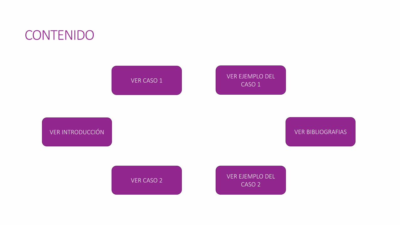
CONTENIDO
VER INTRODUCCIÓN
VER CASO 1
VER CASO 2VER EJEMPLO DEL
CASO 2
VER EJEMPLO DEL CASO 1
VER BIBLIOGRAFIAS
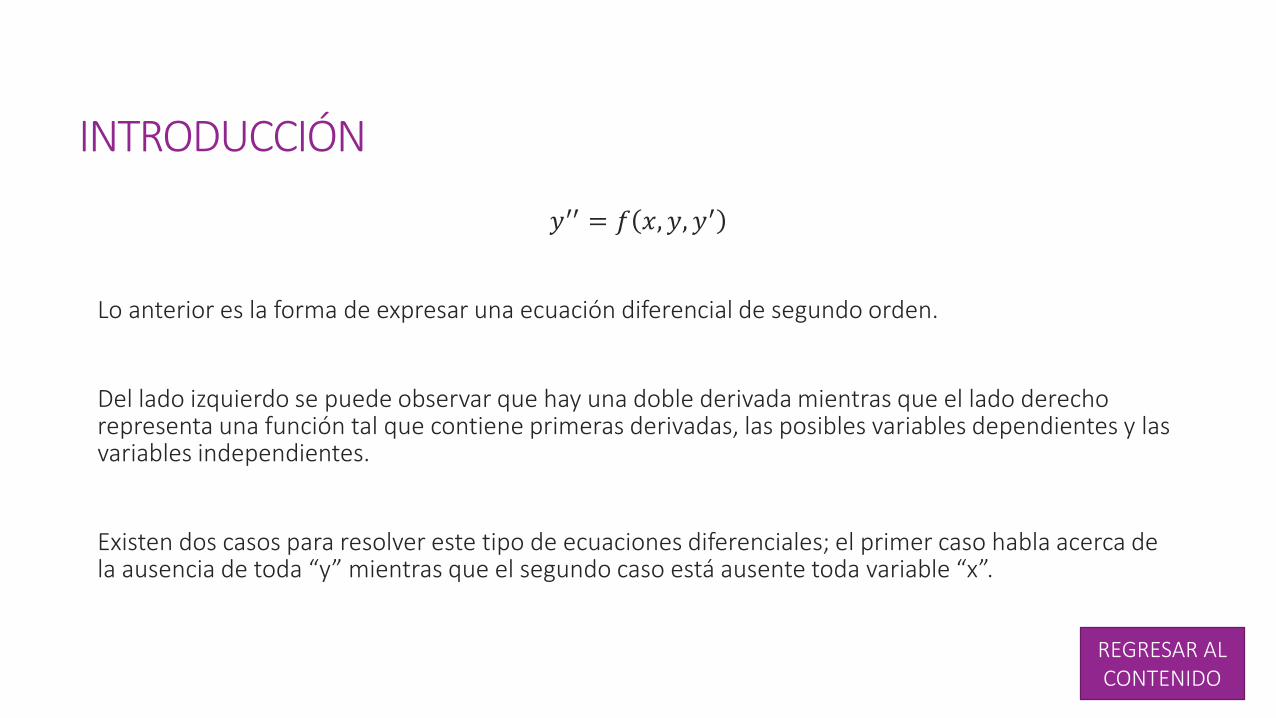
INTRODUCCIÓN
𝑦′′ = 𝑓 𝑥, 𝑦, 𝑦′
Lo anterior es la forma de expresar una ecuación diferencial de segundo orden.
Del lado izquierdo se puede observar que hay una doble derivada mientras que el lado derecho representa una función tal que contiene primeras derivadas, las posibles variables dependientes y las variables independientes.
Existen dos casos para resolver este tipo de ecuaciones diferenciales; el primer caso habla acerca de la ausencia de toda “y” mientras que el segundo caso está ausente toda variable “x”.
REGRESAR AL CONTENIDO
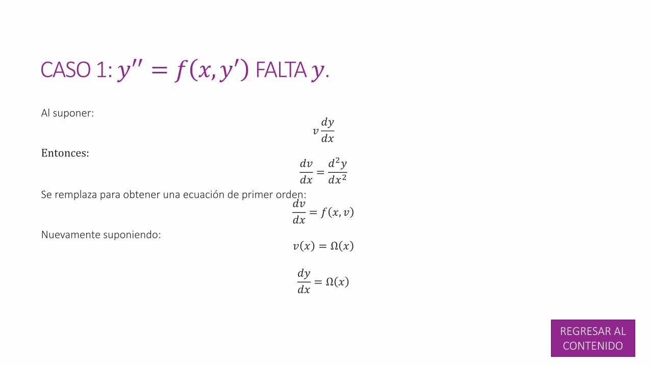
CASO 1: 𝑦′′ = 𝑓 𝑥,𝑦′ FALTA 𝑦.
Al suponer:
𝑣𝑑𝑦
𝑑𝑥
Entonces:𝑑𝑣
𝑑𝑥=𝑑2𝑦
𝑑𝑥2
Se remplaza para obtener una ecuación de primer orden:𝑑𝑣
𝑑𝑥= 𝑓 𝑥, 𝑣
Nuevamente suponiendo:𝑣 𝑥 = Ω 𝑥
𝑑𝑦
𝑑𝑥= Ω 𝑥
REGRESAR AL CONTENIDO
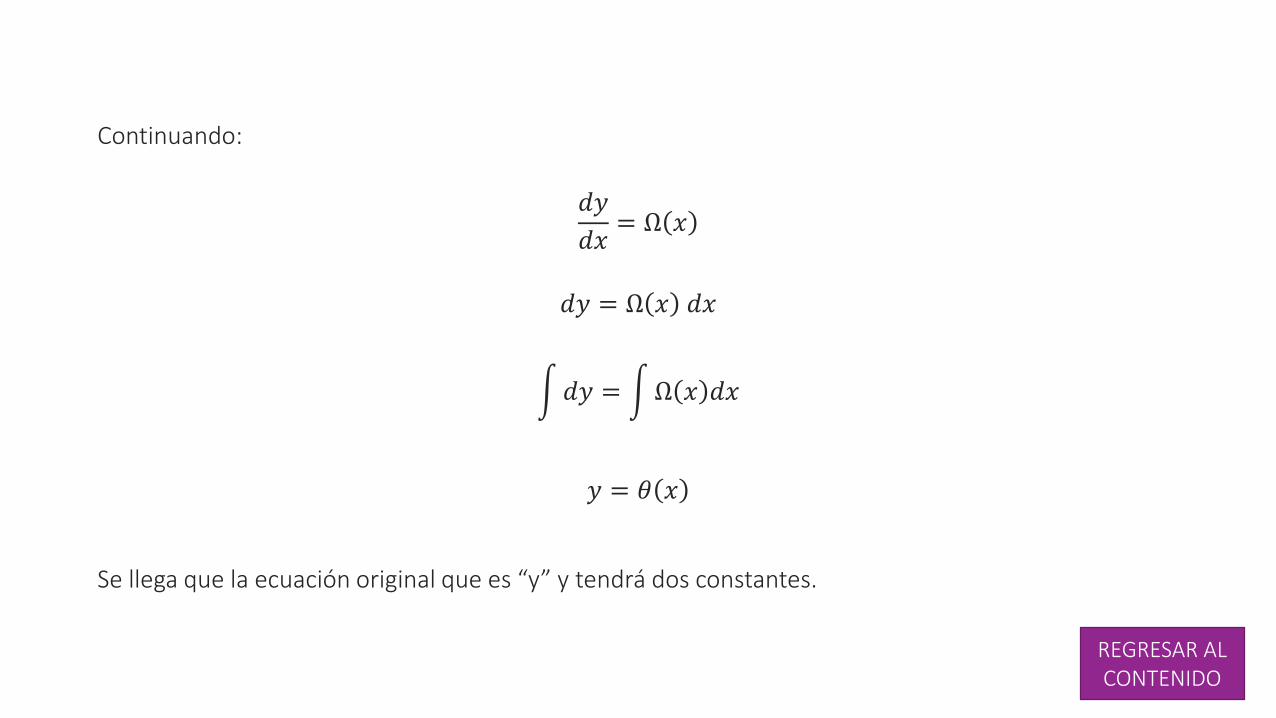
Continuando:
𝑑𝑦
𝑑𝑥= Ω 𝑥
𝑑𝑦 = Ω 𝑥 𝑑𝑥
𝑑𝑦 = Ω 𝑥 𝑑𝑥
𝑦 = 𝜃 𝑥
Se llega que la ecuación original que es “y” y tendrá dos constantes.
REGRESAR AL CONTENIDO
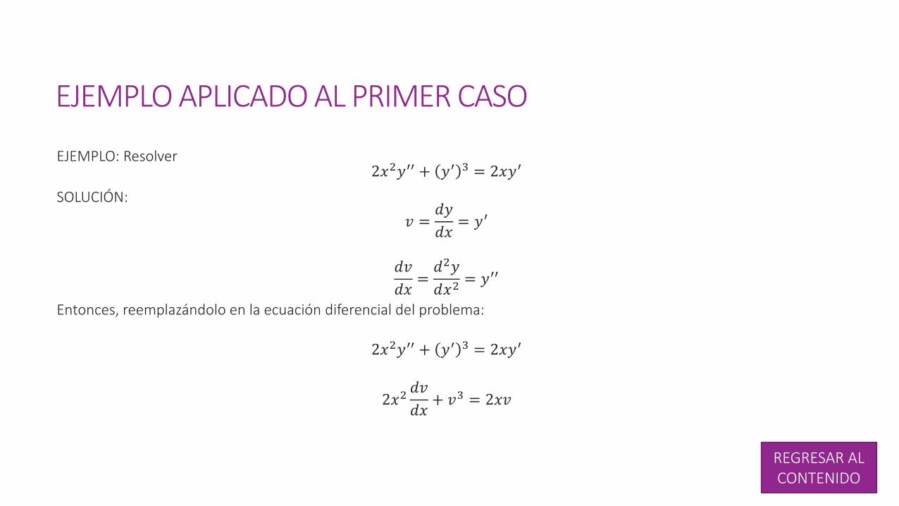
EJEMPLO APLICADO AL PRIMER CASO
EJEMPLO: Resolver2𝑥2𝑦′′ + 𝑦′ 3 = 2𝑥𝑦′
SOLUCIÓN:
𝑣 =𝑑𝑦
𝑑𝑥= 𝑦′
𝑑𝑣
𝑑𝑥=𝑑2𝑦
𝑑𝑥2= 𝑦′′
Entonces, reemplazándolo en la ecuación diferencial del problema:
2𝑥2𝑦′′ + 𝑦′ 3 = 2𝑥𝑦′
2𝑥2𝑑𝑣
𝑑𝑥+ 𝑣3 = 2𝑥𝑣
REGRESAR AL CONTENIDO
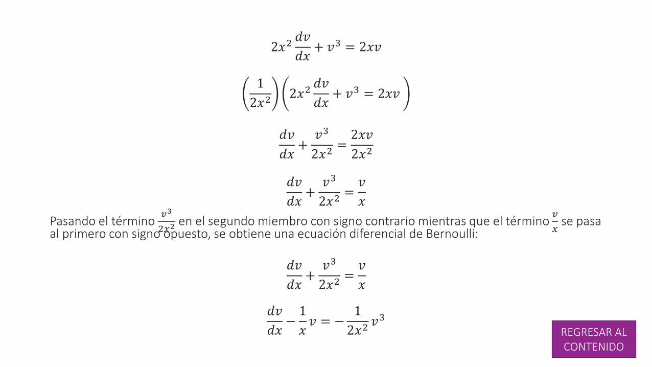
2𝑥2𝑑𝑣
𝑑𝑥+ 𝑣3 = 2𝑥𝑣
1
2𝑥22𝑥2
𝑑𝑣
𝑑𝑥+ 𝑣3 = 2𝑥𝑣
𝑑𝑣
𝑑𝑥+𝑣3
2𝑥2=2𝑥𝑣
2𝑥2
𝑑𝑣
𝑑𝑥+𝑣3
2𝑥2=𝑣
𝑥
Pasando el término 𝑣3
2𝑥2en el segundo miembro con signo contrario mientras que el término
𝑣
𝑥se pasa
al primero con signo opuesto, se obtiene una ecuación diferencial de Bernoulli:
𝑑𝑣
𝑑𝑥+𝑣3
2𝑥2=𝑣
𝑥
𝑑𝑣
𝑑𝑥−1
𝑥𝑣 = −
1
2𝑥2𝑣3
REGRESAR AL CONTENIDO
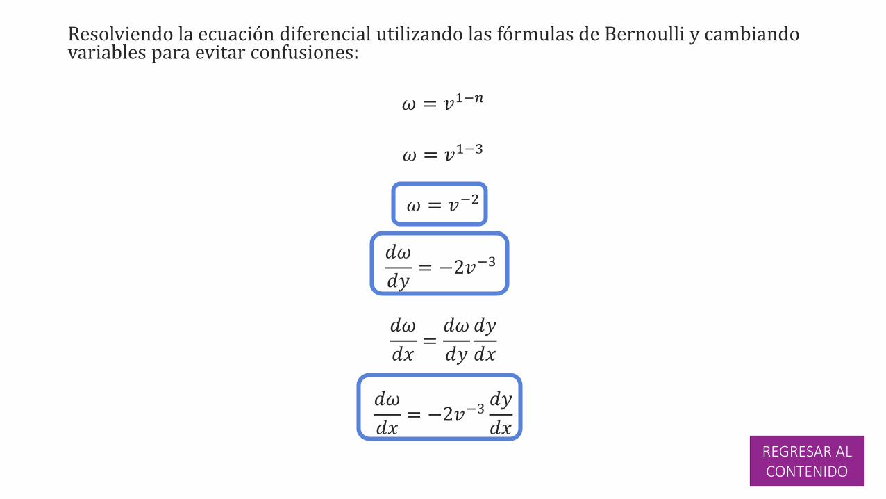
Resolviendo la ecuación diferencial utilizando las fórmulas de Bernoulli y cambiando variables para evitar confusiones:
𝜔 = 𝑣1−𝑛
𝜔 = 𝑣1−3
𝜔 = 𝑣−2
𝑑𝜔
𝑑𝑦= −2𝑣−3
𝑑𝜔
𝑑𝑥=𝑑𝜔
𝑑𝑦
𝑑𝑦
𝑑𝑥
𝑑𝜔
𝑑𝑥= −2𝑣−3
𝑑𝑦
𝑑𝑥REGRESAR AL CONTENIDO
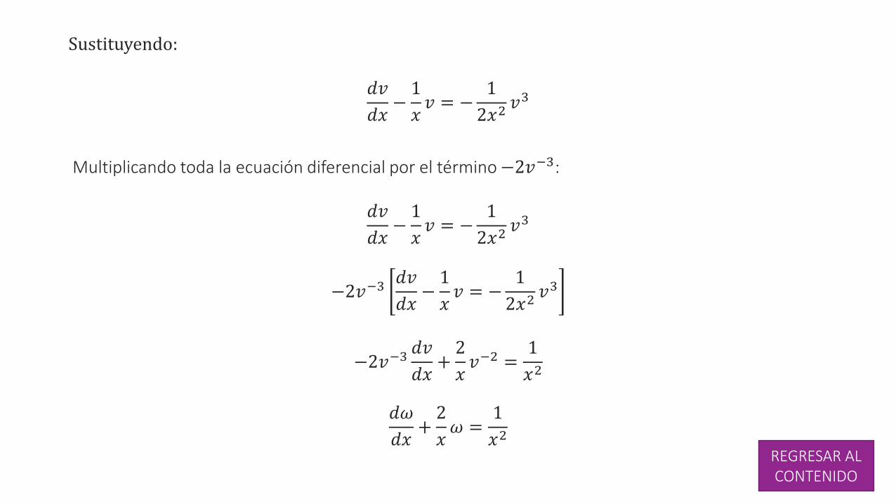
Sustituyendo:
𝑑𝑣
𝑑𝑥−1
𝑥𝑣 = −
1
2𝑥2𝑣3
Multiplicando toda la ecuación diferencial por el término −2𝑣−3:
𝑑𝑣
𝑑𝑥−1
𝑥𝑣 = −
1
2𝑥2𝑣3
−2𝑣−3𝑑𝑣
𝑑𝑥−1
𝑥𝑣 = −
1
2𝑥2𝑣3
−2𝑣−3𝑑𝑣
𝑑𝑥+2
𝑥𝑣−2 =
1
𝑥2
𝑑𝜔
𝑑𝑥+2
𝑥𝜔 =
1
𝑥2REGRESAR AL CONTENIDO
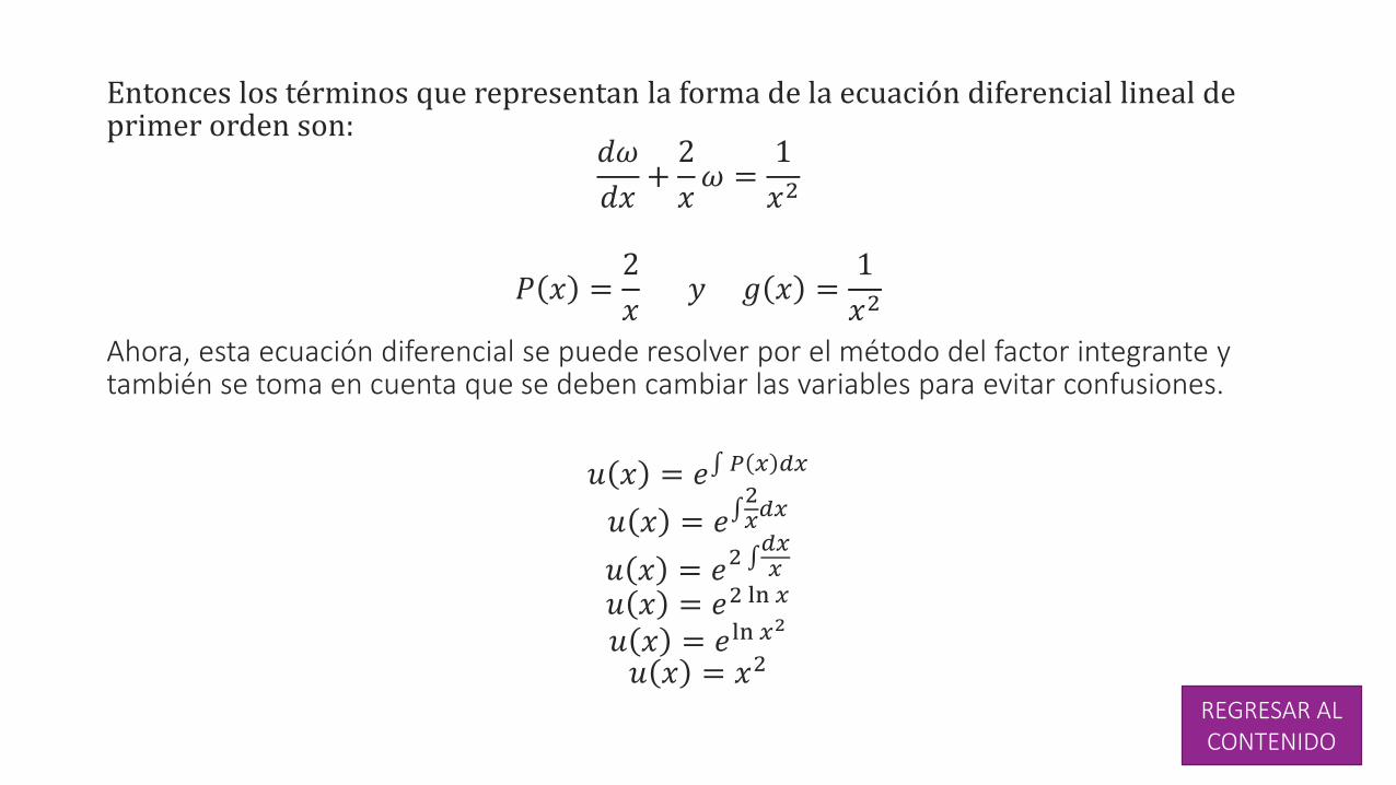
Entonces los términos que representan la forma de la ecuación diferencial lineal de primer orden son:
𝑑𝜔
𝑑𝑥+2
𝑥𝜔 =
1
𝑥2
𝑃 𝑥 =2
𝑥𝑦 𝑔 𝑥 =
1
𝑥2
Ahora, esta ecuación diferencial se puede resolver por el método del factor integrante y también se toma en cuenta que se deben cambiar las variables para evitar confusiones.
𝑢 𝑥 = 𝑒 𝑃 𝑥 𝑑𝑥
𝑢 𝑥 = 𝑒 2𝑥𝑑𝑥
𝑢 𝑥 = 𝑒2 𝑑𝑥𝑥
𝑢 𝑥 = 𝑒2 ln 𝑥
𝑢 𝑥 = 𝑒ln 𝑥2
𝑢 𝑥 = 𝑥2
REGRESAR AL CONTENIDO
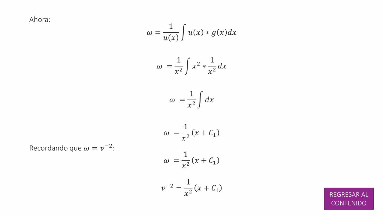
Ahora:
𝜔 =1
𝑢 𝑥 𝑢 𝑥 ∗ 𝑔 𝑥 𝑑𝑥
𝜔 =1
𝑥2 𝑥2 ∗
1
𝑥2𝑑𝑥
𝜔 =1
𝑥2 𝑑𝑥
𝜔 =1
𝑥2𝑥 + 𝐶1
Recordando que 𝜔 = 𝑣−2:
𝜔 =1
𝑥2𝑥 + 𝐶1
𝑣−2 =1
𝑥2𝑥 + 𝐶1
REGRESAR AL CONTENIDO
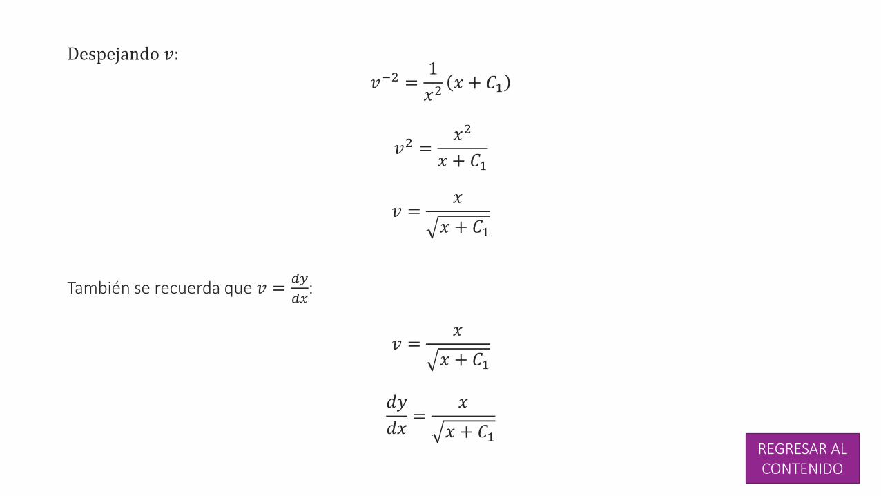
Despejando 𝑣:
𝑣−2 =1
𝑥2𝑥 + 𝐶1
𝑣2 =𝑥2
𝑥 + 𝐶1
𝑣 =𝑥
𝑥 + 𝐶1
También se recuerda que 𝑣 =𝑑𝑦
𝑑𝑥:
𝑣 =𝑥
𝑥 + 𝐶1
𝑑𝑦
𝑑𝑥=
𝑥
𝑥 + 𝐶1REGRESAR AL CONTENIDO
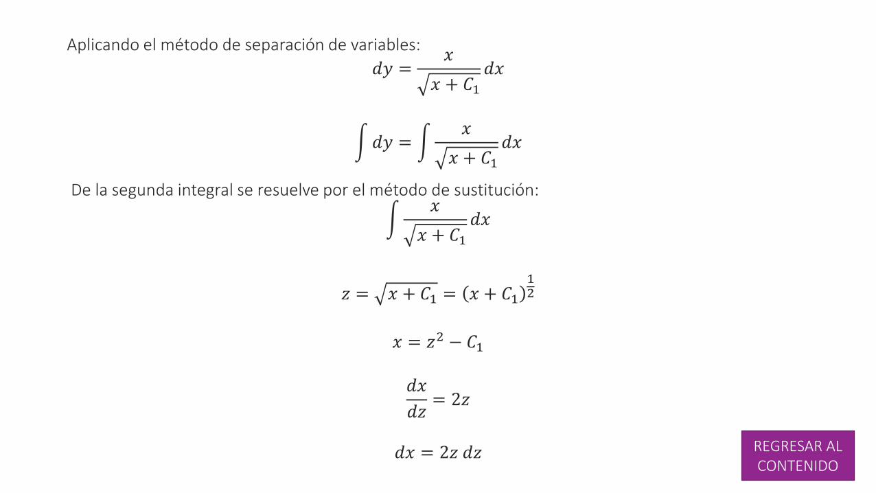
Aplicando el método de separación de variables:
𝑑𝑦 =𝑥
𝑥 + 𝐶1𝑑𝑥
𝑑𝑦 = 𝑥
𝑥 + 𝐶1𝑑𝑥
De la segunda integral se resuelve por el método de sustitución:
𝑥
𝑥 + 𝐶1𝑑𝑥
𝑧 = 𝑥 + 𝐶1 = 𝑥 + 𝐶112
𝑥 = 𝑧2 − 𝐶1
𝑑𝑥
𝑑𝑧= 2𝑧
𝑑𝑥 = 2𝑧 𝑑𝑧 REGRESAR AL CONTENIDO
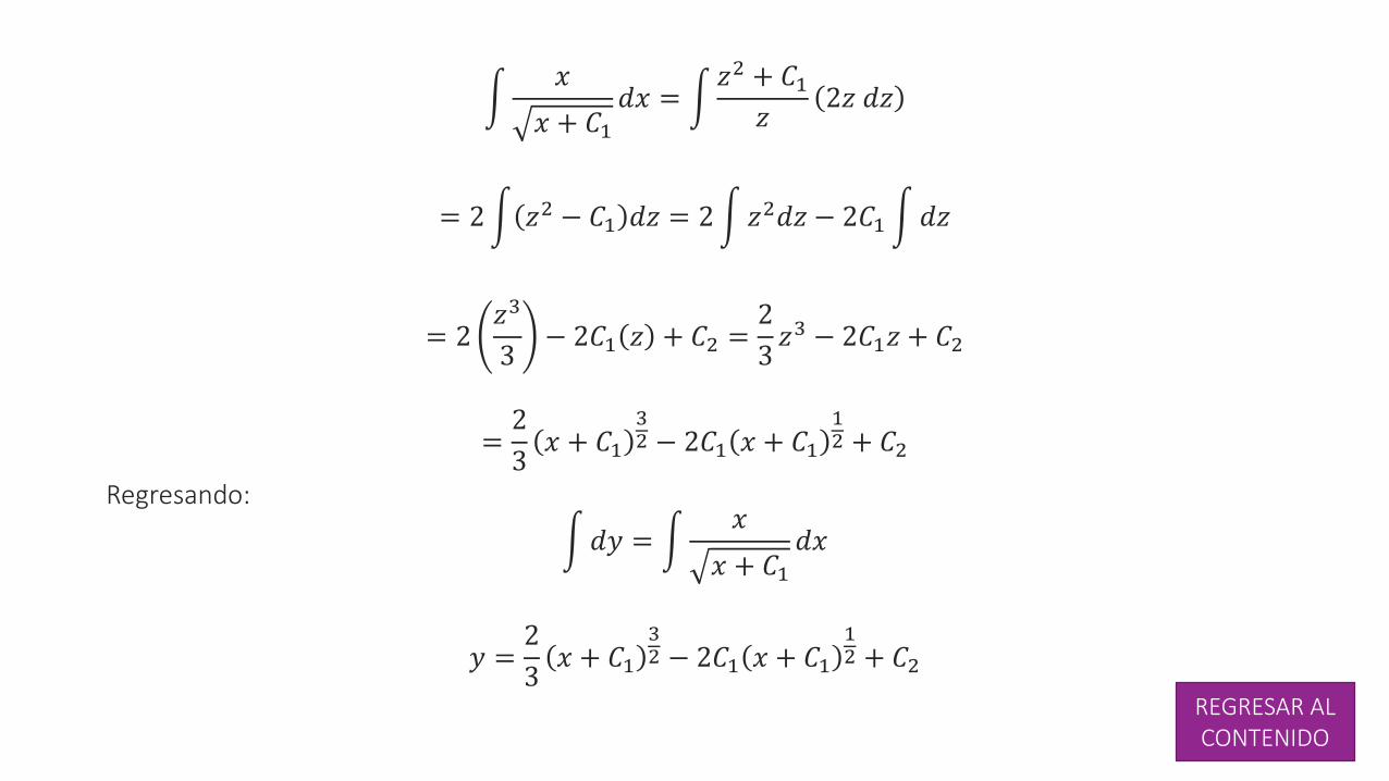
𝑥
𝑥 + 𝐶1𝑑𝑥 =
𝑧2 + 𝐶1𝑧
2𝑧 𝑑𝑧
= 2 𝑧2 − 𝐶1 𝑑𝑧 = 2 𝑧2𝑑𝑧 − 2𝐶1 𝑑𝑧
= 2𝑧3
3− 2𝐶1 𝑧 + 𝐶2 =
2
3𝑧3 − 2𝐶1𝑧 + 𝐶2
=2
3𝑥 + 𝐶1
32 − 2𝐶1 𝑥 + 𝐶1
12 + 𝐶2
Regresando:
𝑑𝑦 = 𝑥
𝑥 + 𝐶1𝑑𝑥
𝑦 =2
3𝑥 + 𝐶1
32 − 2𝐶1 𝑥 + 𝐶1
12 + 𝐶2
REGRESAR AL CONTENIDO
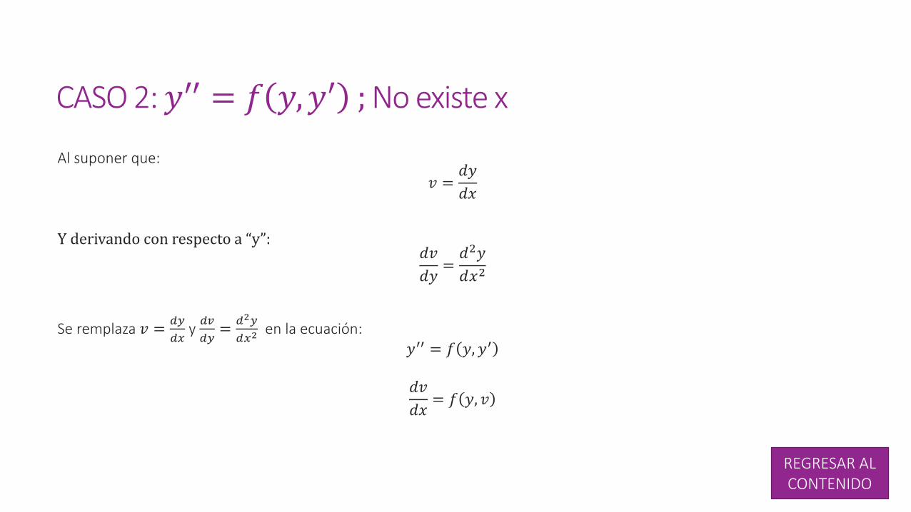
CASO 2: 𝑦′′ = 𝑓 𝑦,𝑦′ ;No existe x
Al suponer que:
𝑣 =𝑑𝑦
𝑑𝑥
Y derivando con respecto a “y”:𝑑𝑣
𝑑𝑦=𝑑2𝑦
𝑑𝑥2
Se remplaza 𝑣 =𝑑𝑦
𝑑𝑥y𝑑𝑣
𝑑𝑦=𝑑2𝑦
𝑑𝑥2en la ecuación:
𝑦′′ = 𝑓 𝑦, 𝑦′
𝑑𝑣
𝑑𝑥= 𝑓 𝑦, 𝑣
REGRESAR AL CONTENIDO
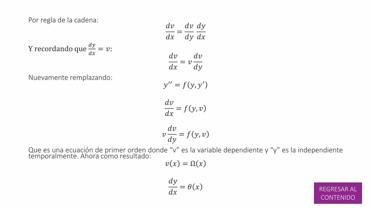
Por regla de la cadena:𝑑𝑣
𝑑𝑥=𝑑𝑣
𝑑𝑦
𝑑𝑦
𝑑𝑥
Y recordando que𝑑𝑦
𝑑𝑥= 𝑣:
𝑑𝑣
𝑑𝑥= 𝑣
𝑑𝑣
𝑑𝑦
Nuevamente remplazando:𝑦′′ = 𝑓 𝑦, 𝑦′
𝑑𝑣
𝑑𝑥= 𝑓 𝑦, 𝑣
𝑣𝑑𝑣
𝑑𝑦= 𝑓 𝑦, 𝑣
Que es una ecuación de primer orden donde “v” es la variable dependiente y “y” es la independientetemporalmente. Ahora como resultado:
𝑣 𝑥 = Ω 𝑥
𝑑𝑦
𝑑𝑥= 𝜃 𝑥 REGRESAR AL
CONTENIDO
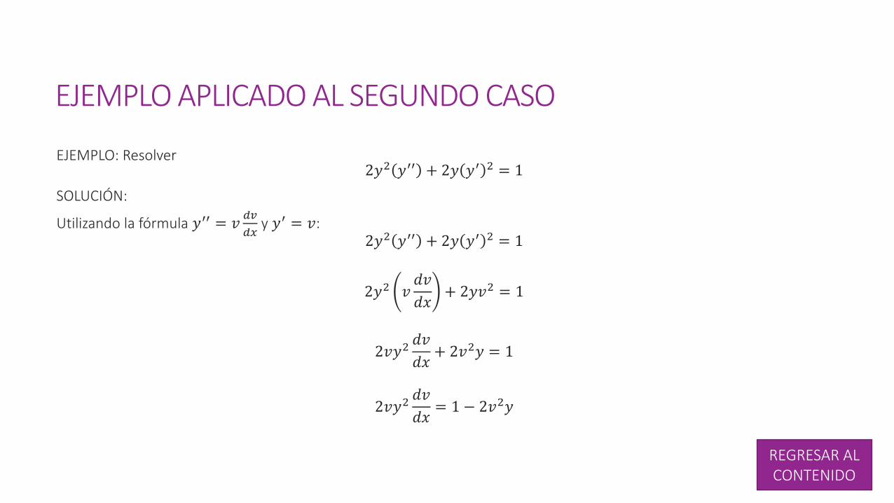
EJEMPLO APLICADO AL SEGUNDO CASO
EJEMPLO: Resolver2𝑦2 𝑦′′ + 2𝑦 𝑦′ 2 = 1
SOLUCIÓN:
Utilizando la fórmula 𝑦′′ = 𝑣𝑑𝑣
𝑑𝑥y 𝑦′ = 𝑣:
2𝑦2 𝑦′′ + 2𝑦 𝑦′ 2 = 1
2𝑦2 𝑣𝑑𝑣
𝑑𝑥+ 2𝑦𝑣2 = 1
2𝑣𝑦2𝑑𝑣
𝑑𝑥+ 2𝑣2𝑦 = 1
2𝑣𝑦2𝑑𝑣
𝑑𝑥= 1 − 2𝑣2𝑦
REGRESAR AL CONTENIDO
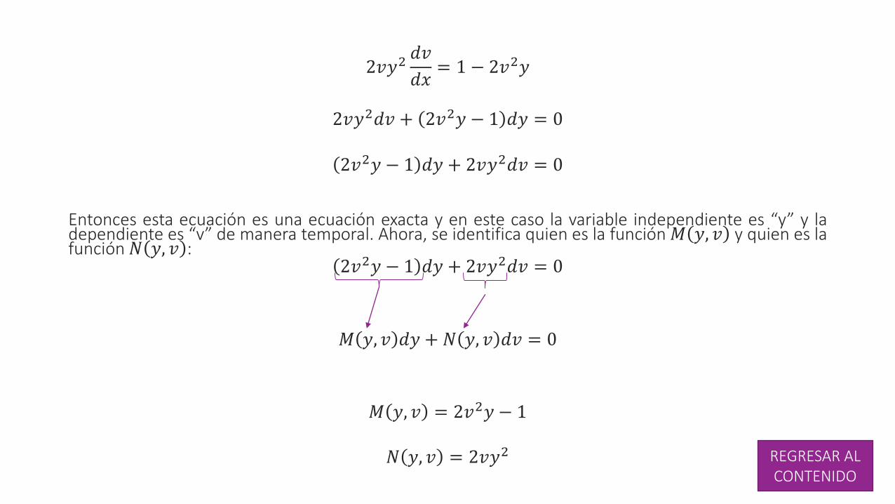
2𝑣𝑦2𝑑𝑣
𝑑𝑥= 1 − 2𝑣2𝑦
2𝑣𝑦2𝑑𝑣 + 2𝑣2𝑦 − 1 𝑑𝑦 = 0
2𝑣2𝑦 − 1 𝑑𝑦 + 2𝑣𝑦2𝑑𝑣 = 0
Entonces esta ecuación es una ecuación exacta y en este caso la variable independiente es “y” y ladependiente es “v” de manera temporal. Ahora, se identifica quien es la función𝑀 𝑦, 𝑣 y quien es lafunción𝑁 𝑦, 𝑣 :
2𝑣2𝑦 − 1 𝑑𝑦 + 2𝑣𝑦2𝑑𝑣 = 0
𝑀 𝑦, 𝑣 𝑑𝑦 + 𝑁 𝑦, 𝑣 𝑑𝑣 = 0
𝑀 𝑦, 𝑣 = 2𝑣2𝑦 − 1
𝑁 𝑦, 𝑣 = 2𝑣𝑦2 REGRESAR AL CONTENIDO
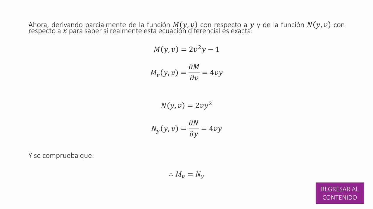
Ahora, derivando parcialmente de la función 𝑀 𝑦, 𝑣 con respecto a 𝑦 y de la función 𝑁 𝑦, 𝑣 conrespecto a 𝑥 para saber si realmente esta ecuación diferencial es exacta:
𝑀 𝑦, 𝑣 = 2𝑣2𝑦 − 1
𝑀𝑣 𝑦, 𝑣 =𝜕𝑀
𝜕𝑣= 4𝑣𝑦
𝑁 𝑦, 𝑣 = 2𝑣𝑦2
𝑁𝑦 𝑦, 𝑣 =𝜕𝑁
𝜕𝑦= 4𝑣𝑦
Y se comprueba que:
∴ 𝑀𝑣 = 𝑁𝑦
REGRESAR AL CONTENIDO
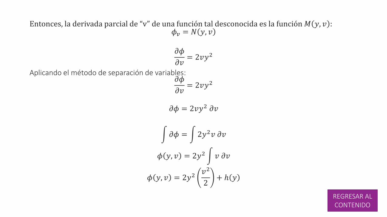
Entonces, la derivada parcial de “v” de una función tal desconocida es la función 𝑀 𝑦, 𝑣 :𝜙𝑣 = 𝑁 𝑦, 𝑣
𝜕𝜙
𝜕𝑣= 2𝑣𝑦2
Aplicando el método de separación de variables:𝜕𝜙
𝜕𝑣= 2𝑣𝑦2
𝜕𝜙 = 2𝑣𝑦2 𝜕𝑣
𝜕𝜙 = 2𝑦2𝑣 𝜕𝑣
𝜙 𝑦, 𝑣 = 2𝑦2 𝑣 𝜕𝑣
𝜙 𝑦, 𝑣 = 2𝑦2𝑣2
2+ ℎ 𝑦
REGRESAR AL CONTENIDO
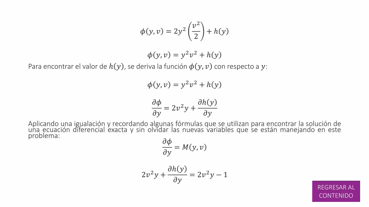
𝜙 𝑦, 𝑣 = 2𝑦2𝑣2
2+ ℎ 𝑦
𝜙 𝑦, 𝑣 = 𝑦2𝑣2 + ℎ 𝑦
Para encontrar el valor de ℎ 𝑦 , se deriva la función 𝜙 𝑦, 𝑣 con respecto a 𝑦:
𝜙 𝑦, 𝑣 = 𝑦2𝑣2 + ℎ 𝑦
𝜕𝜙
𝜕𝑦= 2𝑣2𝑦 +
𝜕ℎ 𝑦
𝜕𝑦
Aplicando una igualación y recordando algunas fórmulas que se utilizan para encontrar la solución deuna ecuación diferencial exacta y sin olvidar las nuevas variables que se están manejando en esteproblema:
𝜕𝜙
𝜕𝑦= 𝑀 𝑦, 𝑣
2𝑣2𝑦 +𝜕ℎ 𝑦
𝜕𝑦= 2𝑣2𝑦 − 1
REGRESAR AL CONTENIDO
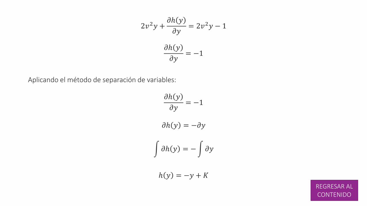
2𝑣2𝑦 +𝜕ℎ 𝑦
𝜕𝑦= 2𝑣2𝑦 − 1
𝜕ℎ 𝑦
𝜕𝑦= −1
Aplicando el método de separación de variables:
𝜕ℎ 𝑦
𝜕𝑦= −1
𝜕ℎ 𝑦 = −𝜕𝑦
𝜕ℎ 𝑦 = − 𝜕𝑦
ℎ 𝑦 = −𝑦 + 𝐾
REGRESAR AL CONTENIDO
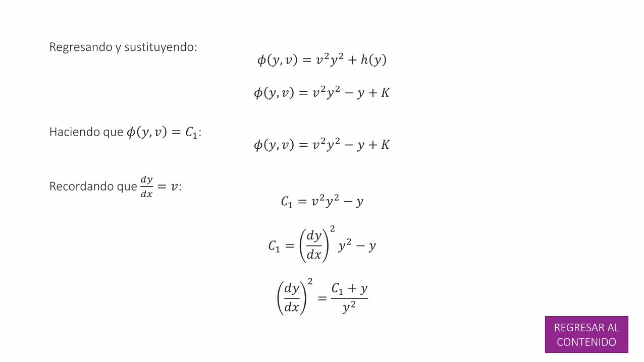
Regresando y sustituyendo:𝜙 𝑦, 𝑣 = 𝑣2𝑦2 + ℎ 𝑦
𝜙 𝑦, 𝑣 = 𝑣2𝑦2 − 𝑦 + 𝐾
Haciendo que 𝜙 𝑦, 𝑣 = 𝐶1:𝜙 𝑦, 𝑣 = 𝑣2𝑦2 − 𝑦 + 𝐾
Recordando que 𝑑𝑦
𝑑𝑥= 𝑣:
𝐶1 = 𝑣2𝑦2 − 𝑦
𝐶1 =𝑑𝑦
𝑑𝑥
2
𝑦2 − 𝑦
𝑑𝑦
𝑑𝑥
2
=𝐶1 + 𝑦
𝑦2
REGRESAR AL CONTENIDO
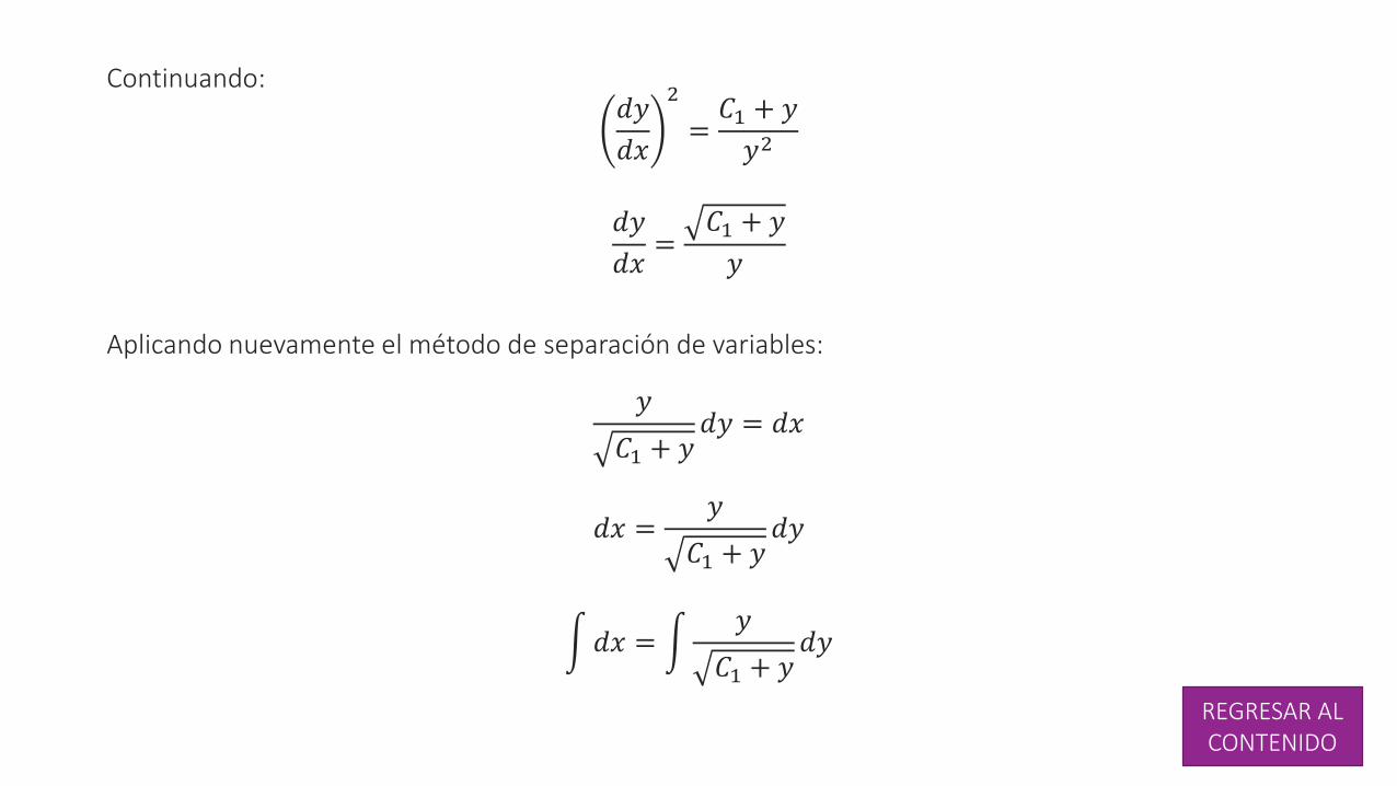
Continuando:𝑑𝑦
𝑑𝑥
2
=𝐶1 + 𝑦
𝑦2
𝑑𝑦
𝑑𝑥=
𝐶1 + 𝑦
𝑦
Aplicando nuevamente el método de separación de variables:
𝑦
𝐶1 + 𝑦𝑑𝑦 = 𝑑𝑥
𝑑𝑥 =𝑦
𝐶1 + 𝑦𝑑𝑦
𝑑𝑥 = 𝑦
𝐶1 + 𝑦𝑑𝑦
REGRESAR AL CONTENIDO
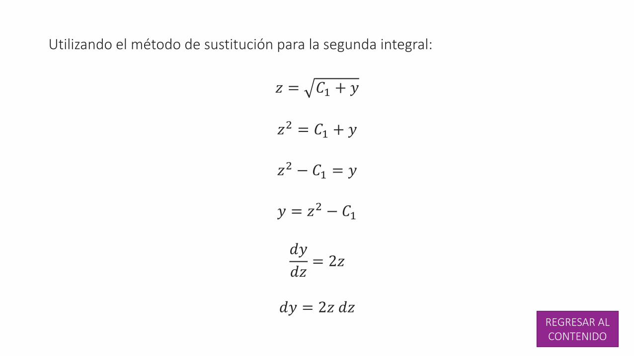
Utilizando el método de sustitución para la segunda integral:
𝑧 = 𝐶1 + 𝑦
𝑧2 = 𝐶1 + 𝑦
𝑧2 − 𝐶1 = 𝑦
𝑦 = 𝑧2 − 𝐶1
𝑑𝑦
𝑑𝑧= 2𝑧
𝑑𝑦 = 2𝑧 𝑑𝑧REGRESAR AL CONTENIDO
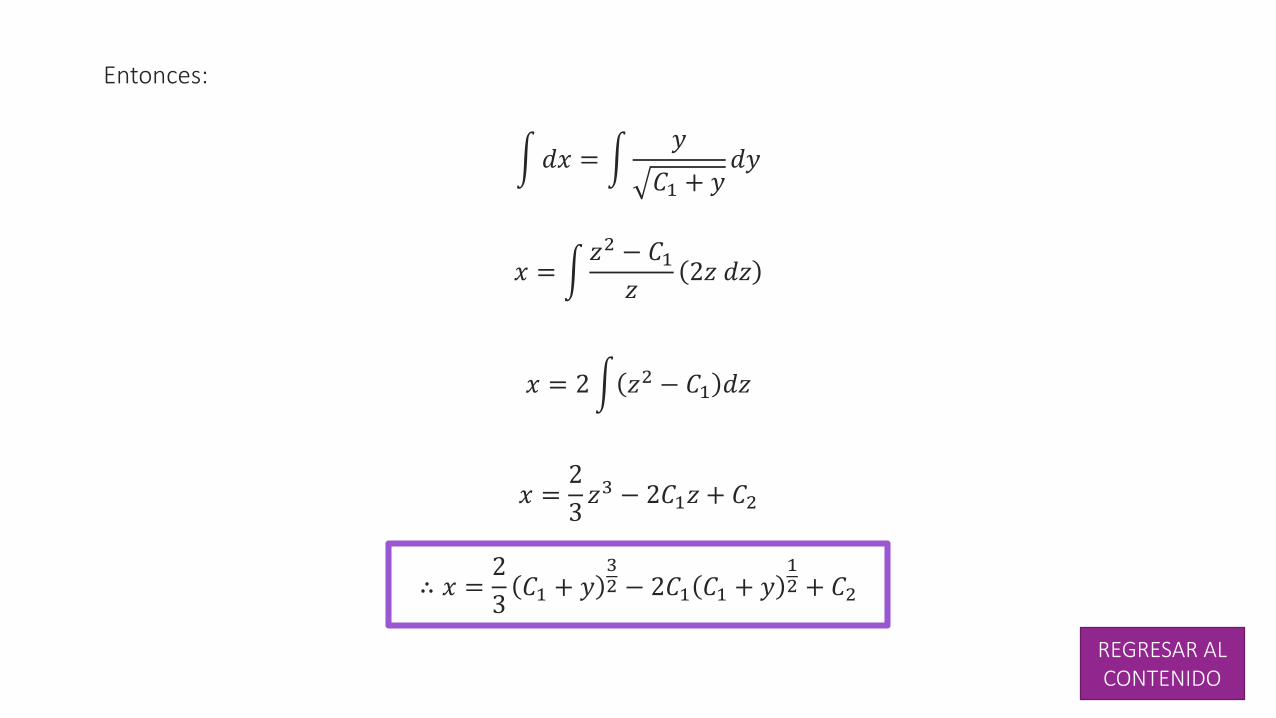
Entonces:
𝑑𝑥 = 𝑦
𝐶1 + 𝑦𝑑𝑦
𝑥 = 𝑧2 − 𝐶1𝑧
2𝑧 𝑑𝑧
𝑥 = 2 𝑧2 − 𝐶1 𝑑𝑧
𝑥 =2
3𝑧3 − 2𝐶1𝑧 + 𝐶2
∴ 𝑥 =2
3𝐶1 + 𝑦
32 − 2𝐶1 𝐶1 + 𝑦
12 + 𝐶2
REGRESAR AL CONTENIDO
BIBLIOGRAFÍASCarmona Jover, I., & Filio López, E. (2011). Ecuaciones diferenciales. México: PEARSON Educación.
D. Zill, D. (2009). Ecuaciones diferenciales con aplicaciones de modelado. México: CENGAGE Learning.
Espinosa Ramos, E. (1996). Ecuaciones diferenciales y sus aplicaciones. Lima.
Jover, I. C. (1998). Ecuaciones diferenciales. México: PEARSON Educación.
REGRESAR AL CONTENIDO