SYMPY:SYMBOLICCOMPUTINGINPYTHON 2 AARON MEURER 1. … · 2017-08-07 · 1 sympy:symboliccomputinginpython 2 aaron meurer∗, christopher p. smith†, mateusz paprocki‡, ondŘej

SYMPY: SYMBOLIC COMPUTING IN PYTHON1

AARON MEURER∗, CHRISTOPHER P. SMITH† , MATEUSZ PAPROCKI‡ , ONDŘEJ2ČERTÍK§ , MATTHEW ROCKLIN¶, AMIT KUMAR‖, SERGIU IVANOV#, JASON K.3MOORE††, SARTAJ SINGH‡‡, THILINA RATHNAYAKE§§, SEAN VIG¶¶, BRIAN E.4

GRANGER‖‖, RICHARD P. MULLER##, FRANCESCO BONAZZI1, HARSH GUPTA2,5SHIVAM VATS3, FREDRIK JOHANSSON4, FABIAN PEDREGOSA5, MATTHEW J.6CURRY6, ASHUTOSH SABOO7, ISURU FERNANDO8, SUMITH KULAL9, ROBERT7

CIMRMAN10, AND ANTHONY SCOPATZ118

Abstract. SymPy is an open source computer algebra system written in pure Python. It9is built with a focus on extensibility and ease of use, through both interactive and programmatic10applications. These characteristics have led SymPy to become the standard symbolic library for11the scientific Python ecosystem. This paper presents the architecture of SymPy, a description of its12features, and a discussion of select domain specific submodules.13

1. Introduction. SymPy is a full featured computer algebra system (CAS) writ-14ten in the Python programming language [24]. It is free and open source software,15being licensed under the 3-clause BSD license [36]. The SymPy project was started16

∗University of South Carolina, Columbia, SC 29201 ([email protected]).†Polar Semiconductor, Inc., Bloomington, MN 55425 ([email protected]).‡Continuum Analytics, Inc., Austin, TX 78701 ([email protected]).§Los Alamos National Laboratory, Los Alamos, NM 87545 ([email protected]).¶Continuum Analytics, Inc., Austin, TX 78701 ([email protected]).‖Delhi Technological University, Shahbad Daulatpur, Bawana Road, New Delhi 110042, India

([email protected]).#Université Paris Est Créteil, 61 av. Général de Gaulle, 94010 Créteil, France (sergiu.ivanov@u-

pec.fr).††University of California, Davis, Davis, CA 95616 ([email protected]).‡‡Indian Institute of Technology (BHU), Varanasi, Uttar Pradesh 221005, India (singhsar-

[email protected]).§§University of Moratuwa, Bandaranayake Mawatha, Katubedda, Moratuwa 10400, Sri Lanka

([email protected]).¶¶University of Illinois at Urbana-Champaign, Urbana, IL 61801 ([email protected]).‖‖California Polytechnic State University, San Luis Obispo, CA 93407 ([email protected]).

##Center for Computing Research, Sandia National Laboratories, Albuquerque, NM 87185([email protected]).

1Max Planck Institute of Colloids and Interfaces, Department of Theory and Bio-Systems, AmMühlenberg 1, 14424 Potsdam, Germany ([email protected]).

2Indian Institute of Technology Kharagpur, Kharagpur, West Bengal 721302, India ([email protected]).

3Indian Institute of Technology Kharagpur, Kharagpur, West Bengal 721302, India ([email protected]).

4INRIA Bordeaux-Sud-Ouest – LFANT project-team, 200 Avenue de la Vieille Tour, 33405 Tal-ence, France ([email protected]).

5INRIA – SIERRA project-team, 2 Rue Simone IFF, 75012 Paris, France ([email protected]).6Department of Physics and Astronomy, University of New Mexico, Albuquerque, NM 87131

([email protected]).7Birla Institute of Technology and Science, Pilani, K.K. Birla Goa Campus, NH 17B Bypass

Road, Zuarinagar, Sancoale, Goa 403726, India ([email protected]).8University of Moratuwa, Bandaranayake Mawatha, Katubedda, Moratuwa 10400, Sri Lanka

([email protected]).9Indian Institute of Technology Bombay, Powai, Mumbai, Maharashtra 400076, India (sum-

[email protected]).10New Technologies – Research Centre, University of West Bohemia, Univerzitní 8, 306 14 Plzeň,

Czech Republic ([email protected]).11University of South Carolina, Columbia, SC 29201 ([email protected]).

1

This manuscript is for review purposes only.PeerJ Preprints | https://doi.org/10.7287/peerj.preprints.2083v2 | CC-BY 4.0 Open Access | rec: 30 May 2016, publ: 30 May 2016

mailto:[email protected]





























by Ondřej Čertík in 2005, and it has since grown to over 500 contributors. Currently,17SymPy is developed on GitHub using a bazaar community model [32]. The accessibil-18ity of the codebase and the open community model allow SymPy to rapidly respond19to the needs of users and developers.20

Python is a dynamically typed programming language that has a focus on ease21of use and readability. Due in part to this focus, it has become a popular language22for scientific computing and data science, with a broad ecosystem of libraries [27].23SymPy is itself used by many libraries and tools to support research within a variety of24domains, such as Sage [39] (pure mathematics), yt [44] (astronomy and astrophysics),25PyDy [15] (multibody dynamics), and SfePy [10] (finite elements).26

Unlike many CASs, SymPy does not invent its own programming language.27Python itself is used both for the internal implementation and end user interaction.28The exclusive usage of a single programming language makes it easier for people al-29ready familiar with that language to use or develop SymPy. Simultaneously, it enables30developers to focus on mathematics, rather than language design.31

SymPy is designed with a strong focus on usability as a library. Extensibility is32important in its application program interface (API) design. Thus, SymPy makes no33attempt to extend the Python language itself. The goal is for users of SymPy to be34able to include SymPy alongside other Python libraries in their workflow, whether35that be in an interactive environment or as a programmatic part in a larger system.36

As a library, SymPy does not have a built-in graphical user interface (GUI). How-37ever, SymPy exposes a rich interactive display system, including registering printers38with Jupyter [29] frontends, including the Notebook and Qt Console, which will render39SymPy expressions using MathJax [9] or LATEX.40

The remainder of this paper discusses key components of the SymPy software.41Section 2 discusses the architecture of SymPy. Section 3 enumerates the features of42SymPy and takes a closer look at some of the important ones. The section 4 looks at43the numerical features of SymPy and its dependency library, mpmath. Section 5 looks44at the domain specific physics submodules for performing symbolic and numerical45calculations in classical mechanics and quantum mechanics. Conclusions and future46directions for SymPy are given in section 6.47

2. Architecture. Software architecture is of central importance in any large48software project because it establishes predictable patterns of usage and develop-49ment [38]. This section describes the essential structural components of SymPy, pro-50vides justifications for the design decisions that have been made, and gives example51user-facing code as appropriate.52

2.1. Basic Usage. The following statement imports all SymPy functions into53the global Python namespace. From here on, all examples in this paper assume that54this statement has been executed.55>>> from sympy import *56

Symbolic variables, called symbols, must be defined and assigned to Python vari-57ables before they can be used. This is typically done through the symbols function,58which may create multiple symbols in a single function call. For instance,59>>> x, y, z = symbols('x y z')60creates three symbols representing variables named x, y, and z. In this particular in-61stance, these symbols are all assigned to Python variables of the same name. However,62the user is free to assign them to different Python variables, while representing the63same symbol, such as a, b, c = symbols('x y z'). In order to minimize potential64confusion, though, all examples in this paper will assume that the symbols x, y, and65

2


z have been assigned to Python variables identical to their symbolic names.66Expressions are created from symbols using Python’s mathematical syntax. Note67

that in Python, exponentiation is represented by the ** binary infix operator. For68instance, the following Python code creates the expression (x2 − 2x+ 3)/y.69>>> (x**2 - 2*x + 3)/y70(x**2 - 2*x + 3)/y71

Importantly, SymPy expressions are immutable. This simplifies the design of72SymPy by allowing expression interning. It also enables expressions to be hashed and73stored in Python dictionaries, thereby permitting features such as caching.74

2.2. The Core. A computer algebra system (CAS) represents mathematical75expressions as data structures. For example, the mathematical expression x + y is76represented as a tree with three nodes, +, x, and y, where x and y are ordered children77of +. As users manipulate mathematical expressions with traditional mathematical78syntax, the CAS manipulates the underlying data structures. Automated optimiza-79tions and computations such as integration, simplification, etc. are all functions that80consume and produce expression trees.81

In SymPy every symbolic expression is an instance of a Python Basic class, a82superclass of all SymPy types providing common methods to all SymPy tree-elements,83such as traversals. The children of a node in the tree are held in the args attribute.84A terminal or leaf node in the expression tree has empty args.85

For example, consider the expression xy + 2:86>>> expr = x*y + 287By order of operations, the parent of the expression tree for expr is an addition, so it88is of type Add. The child nodes of expr are 2 and x*y.89>>> type(expr)90<class 'sympy.core.add.Add'>91>>> expr.args92(2, x*y)93

Descending further down into the expression tree yields the full expression. For94example, the next child node (given by expr.args[0]) is 2. Its class is Integer, and95it has an empty args tuple, indicating that it is a leaf node.96>>> expr.args[0]97298>>> type(expr.args[0])99<class 'sympy.core.numbers.Integer'>100>>> expr.args[0].args101()102

A useful way to view an expression tree is using the srepr function, which returns103a string representation of an expression as valid Python code with all the nested class104constructor calls to create the given expression.105>>> srepr(expr)106"Add(Mul(Symbol('x'), Symbol('y')), Integer(2))"107

Every SymPy expression satisfies a key identity invariant:108expr.func(*expr.args) == expr109This means that expressions are rebuildable from their args.1 Note that in SymPy110the == operator represents exact structural equality, not mathematical equality. This111allows testing if any two expressions are equal to one another as expression trees. For112

1expr.func is used instead of type(expr) to allow the function of an expression to be distinct fromits actual Python class. In most cases the two are the same.

3


example, even though (x+ 1)2 and x2 +2x+1 are equal mathematically, SymPy gives113>>> (x + 1)**2 == x**2 + 2*x + 1114False115because they are different as expression trees (the former is a Pow object and the latter116is an Add object).117

Python allows classes to override mathematical operators. The Python interpreter118translates the above x*y + 2 to, roughly, (x.__mul__(y)).__add__(2). Both x and y,119returned from the symbols function, are Symbol instances. The 2 in the expression is120processed by Python as a literal, and is stored as Python’s built in int type. When 2 is121passed to the __add__ method of Symbol, it is converted to the SymPy type Integer(2)122before being stored in the resulting expression tree. In this way, SymPy expressions123can be built in the natural way using Python operators and numeric literals.124

2.3. Assumptions. SymPy performs logical inference through its assumptions125system. The assumptions system allows users to specify that symbols have cer-126tain common mathematical properties, such as being positive, imaginary, or integral.127SymPy is careful to never perform simplifications on an expression unless the assump-128tions allow them. For instance, the identity

√t2 = t holds if t is nonnegative (t ≥ 0).129

If t is real, the identity√t2 = |t| holds. However, for general complex t, no such130

identity holds.131By default, SymPy performs all calculations assuming that symbols are com-132

plex valued. This assumption makes it easier to treat mathematical problems in full133generality.134>>> t = Symbol('t')135>>> sqrt(t**2)136sqrt(t**2)137

By assuming the most general case, that symbols are complex by default, SymPy138avoids performing mathematically invalid operations. However, in many cases users139will wish to simplify expressions containing terms like

√t2.140

Assumptions are set on Symbol objects when they are created. For instance141Symbol('t', positive=True) will create a symbol named t that is assumed to be142positive.143>>> t = Symbol('t', positive=True)144>>> sqrt(t**2)145t146

Some of the common assumptions that SymPy allows are positive, negative,147real, nonpositive, nonnegative, real, integer, and commutative.2 Assumptions on148any object can be checked with the is_assumption attributes, like t.is_positive.149

Assumptions are only needed to restrict a domain so that certain simplifications150can be performed. They are not required to make the domain match the input of a151function. For instance, one can create the object

∑mn=0 f(n) as Sum(f(n), (n, 0, m))152

without setting integer=True when creating the Symbol object n.153The assumptions system additionally has deductive capabilities. The assump-154

tions use a three-valued logic using the Python built in objects True, False, and155None. None represents the “unknown” case. This could mean that given assumptions156do not unambiguously specify the truth of an attribute. For instance, Symbol('x',157real=True).is_positive will give None because a real symbol might be positive or neg-158ative. The None could also mean that not enough is known or implemented to compute159

2If A and B are Symbols created with commutative=False then SymPy will keep A · B and B · Adistinct.

4


the given fact. For instance, (pi + E).is_irrational gives None, because determining160whether π + e is rational or irrational is an open problem in mathematics [23].161

Basic implications between the facts are used to deduce assumptions. For in-162stance, the assumptions system knows that being an integer implies being rational,163so Symbol('x', integer=True).is_rational returns True. Furthermore, expressions164compute the assumptions on themselves based on the assumptions of their argu-165ments. For instance, if x and y are both created with positive=True, then (x +166y).is_positive will be True whereas (x - y).is_positive will be None.167

2.4. Extensibility. While the core of SymPy is relatively small, it has been168extended to a wide variety of domains by a broad range of contributors. This is due in169part because the same language, Python, is used both for the internal implementation170and the external usage by users. All of the extensibility capabilities available to users171are also utilized by SymPy itself. This eases the transition pathway from SymPy user172to SymPy developer.173

The typical way to create a custom SymPy object is to subclass an existing SymPy174class, usually Basic, Expr, or Function. All SymPy classes used for expression trees3175should be subclasses of the base class Basic, which defines some basic methods for176symbolic expression trees. Expr is the subclass for mathematical expressions that177can be added and multiplied together. Instances of Expr typically represent complex178numbers, but may also include other “rings” like matrix expressions. Not all SymPy179classes are subclasses of Expr. For instance, logic expressions such as And(x, y) are180subclasses of Basic but not of Expr.181

The Function class is a subclass of Expr which makes it easier to define mathe-182matical functions called with arguments. This includes named functions like sin(x)183and log(x) as well as undefined functions like f(x). Subclasses of Function should184define a class method eval, which returns values for which the function should be185automatically evaluated, and None for arguments that should not be automatically186evaluated.187

Many SymPy functions perform various evaluations down the expression tree.188Classes define their behavior in such functions by defining a relevant _eval_* method.189For instance, an object can indicate to the diff function how to take the derivative190of itself by defining the _eval_derivative(self, x) method, which may in turn call191diff on its args. The most common _eval_* methods relate to the assumptions.192_eval_is_assumption defines the assumptions for assumption.193

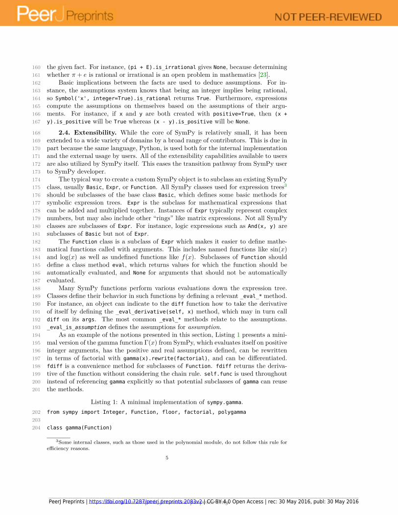
As an example of the notions presented in this section, Listing 1 presents a mini-194mal version of the gamma function Γ(x) from SymPy, which evaluates itself on positive195integer arguments, has the positive and real assumptions defined, can be rewritten196in terms of factorial with gamma(x).rewrite(factorial), and can be differentiated.197fdiff is a convenience method for subclasses of Function. fdiff returns the deriva-198tive of the function without considering the chain rule. self.func is used throughout199instead of referencing gamma explicitly so that potential subclasses of gamma can reuse200the methods.201

Listing 1: A minimal implementation of sympy.gamma.from sympy import Integer, Function, floor, factorial, polygamma202

203class gamma(Function)204

3Some internal classes, such as those used in the polynomial module, do not follow this rule forefficiency reasons.

5


@classmethod205def eval(cls, arg):206

if isinstance(arg, Integer) and arg.is_positive:207return factorial(arg - 1)208

209def _eval_is_positive(self):210

x = self.args[0]211if x.is_positive:212

return True213elif x.is_noninteger:214

return floor(x).is_even215216

def _eval_is_real(self):217x = self.args[0]218# noninteger means real and not integer219if x.is_positive or x.is_noninteger:220

return True221222

def _eval_rewrite_as_factorial(self, z):223return factorial(z - 1)224

225def fdiff(self, argindex=1):226

from sympy.core.function import ArgumentIndexError227if argindex == 1:228

return self.func(self.args[0])*polygamma(0, self.args[0])229else:230

raise ArgumentIndexError(self, argindex)231

The gamma function implemented in SymPy has many more capabilities than the232above listing, such as evaluation at rational points and series expansion.233

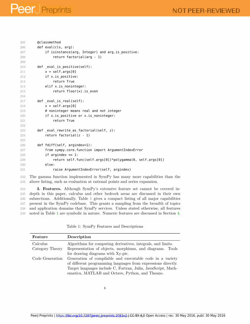
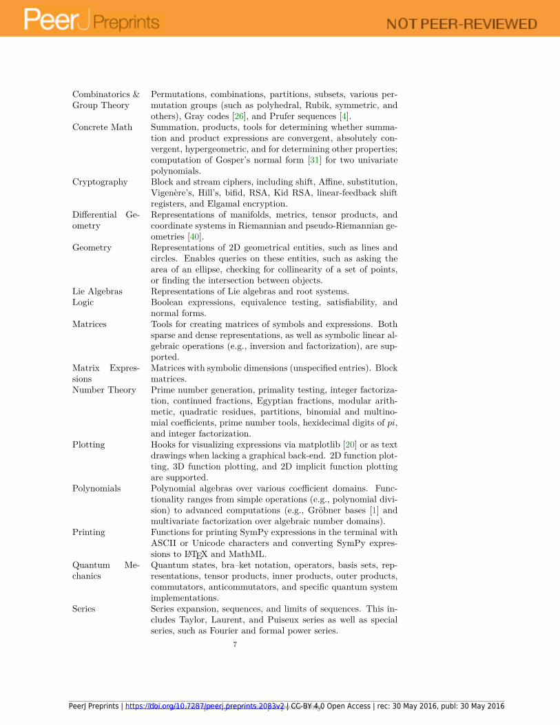
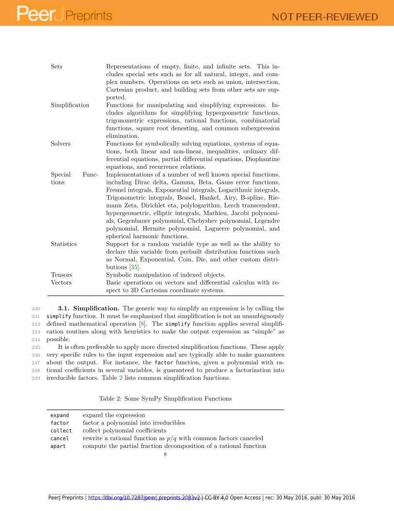
3. Features. Although SymPy’s extensive feature set cannot be covered in-234depth in this paper, calculus and other bedrock areas are discussed in their own235subsections. Additionally, Table 1 gives a compact listing of all major capabilities236present in the SymPy codebase. This grants a sampling from the breadth of topics237and application domains that SymPy services. Unless stated otherwise, all features238noted in Table 1 are symbolic in nature. Numeric features are discussed in Section 4.239

Table 1: SymPy Features and Descriptions

Feature DescriptionCalculus Algorithms for computing derivatives, integrals, and limits.Category Theory Representation of objects, morphisms, and diagrams. Tools

for drawing diagrams with Xy-pic.Code Generation Generation of compilable and executable code in a variety

of different programming languages from expressions directly.Target languages include C, Fortran, Julia, JavaScript, Math-ematica, MATLAB and Octave, Python, and Theano.

6


Combinatorics &Group Theory

Permutations, combinations, partitions, subsets, various per-mutation groups (such as polyhedral, Rubik, symmetric, andothers), Gray codes [26], and Prufer sequences [4].

Concrete Math Summation, products, tools for determining whether summa-tion and product expressions are convergent, absolutely con-vergent, hypergeometric, and for determining other properties;computation of Gosper’s normal form [31] for two univariatepolynomials.

Cryptography Block and stream ciphers, including shift, Affine, substitution,Vigenère’s, Hill’s, bifid, RSA, Kid RSA, linear-feedback shiftregisters, and Elgamal encryption.

Differential Ge-ometry

Representations of manifolds, metrics, tensor products, andcoordinate systems in Riemannian and pseudo-Riemannian ge-ometries [40].

Geometry Representations of 2D geometrical entities, such as lines andcircles. Enables queries on these entities, such as asking thearea of an ellipse, checking for collinearity of a set of points,or finding the intersection between objects.

Lie Algebras Representations of Lie algebras and root systems.Logic Boolean expressions, equivalence testing, satisfiability, and

normal forms.Matrices Tools for creating matrices of symbols and expressions. Both

sparse and dense representations, as well as symbolic linear al-gebraic operations (e.g., inversion and factorization), are sup-ported.

Matrix Expres-sions

Matrices with symbolic dimensions (unspecified entries). Blockmatrices.

Number Theory Prime number generation, primality testing, integer factoriza-tion, continued fractions, Egyptian fractions, modular arith-metic, quadratic residues, partitions, binomial and multino-mial coefficients, prime number tools, hexidecimal digits of pi,and integer factorization.

Plotting Hooks for visualizing expressions via matplotlib [20] or as textdrawings when lacking a graphical back-end. 2D function plot-ting, 3D function plotting, and 2D implicit function plottingare supported.

Polynomials Polynomial algebras over various coefficient domains. Func-tionality ranges from simple operations (e.g., polynomial divi-sion) to advanced computations (e.g., Gröbner bases [1] andmultivariate factorization over algebraic number domains).

Printing Functions for printing SymPy expressions in the terminal withASCII or Unicode characters and converting SymPy expres-sions to LATEX and MathML.

Quantum Me-chanics

Quantum states, bra–ket notation, operators, basis sets, rep-resentations, tensor products, inner products, outer products,commutators, anticommutators, and specific quantum systemimplementations.

Series Series expansion, sequences, and limits of sequences. This in-cludes Taylor, Laurent, and Puiseux series as well as specialseries, such as Fourier and formal power series.

7


Sets Representations of empty, finite, and infinite sets. This in-cludes special sets such as for all natural, integer, and com-plex numbers. Operations on sets such as union, intersection,Cartesian product, and building sets from other sets are sup-ported.

Simplification Functions for manipulating and simplifying expressions. In-cludes algorithms for simplifying hypergeometric functions,trigonometric expressions, rational functions, combinatorialfunctions, square root denesting, and common subexpressionelimination.

Solvers Functions for symbolically solving equations, systems of equa-tions, both linear and non-linear, inequalities, ordinary dif-ferential equations, partial differential equations, Diophantineequations, and recurrence relations.

Special Func-tions

Implementations of a number of well known special functions,including Dirac delta, Gamma, Beta, Gauss error functions,Fresnel integrals, Exponential integrals, Logarithmic integrals,Trigonometric integrals, Bessel, Hankel, Airy, B-spline, Rie-mann Zeta, Dirichlet eta, polylogarithm, Lerch transcendent,hypergeometric, elliptic integrals, Mathieu, Jacobi polynomi-als, Gegenbauer polynomial, Chebyshev polynomial, Legendrepolynomial, Hermite polynomial, Laguerre polynomial, andspherical harmonic functions.

Statistics Support for a random variable type as well as the ability todeclare this variable from prebuilt distribution functions suchas Normal, Exponential, Coin, Die, and other custom distri-butions [35].

Tensors Symbolic manipulation of indexed objects.Vectors Basic operations on vectors and differential calculus with re-

spect to 3D Cartesian coordinate systems.

3.1. Simplification. The generic way to simplify an expression is by calling the240simplify function. It must be emphasized that simplification is not an unambiguously241defined mathematical operation [8]. The simplify function applies several simplifi-242cation routines along with heuristics to make the output expression as “simple” as243possible.244

It is often preferable to apply more directed simplification functions. These apply245very specific rules to the input expression and are typically able to make guarantees246about the output. For instance, the factor function, given a polynomial with ra-247tional coefficients in several variables, is guaranteed to produce a factorization into248irreducible factors. Table 2 lists common simplification functions.249

Table 2: Some SymPy Simplification Functions

expand expand the expressionfactor factor a polynomial into irreduciblescollect collect polynomial coefficientscancel rewrite a rational function as p/q with common factors canceledapart compute the partial fraction decomposition of a rational function

8


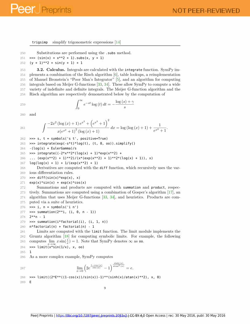
trigsimp simplify trigonometric expressions [14]

Substitutions are performed using the .subs method.250>>> (sin(x) + x**2 + 1).subs(x, y + 1)251(y + 1)**2 + sin(y + 1) + 1252

3.2. Calculus. Integrals are calculated with the integrate function. SymPy im-253plements a combination of the Risch algorithm [6], table lookups, a reimplementation254of Manuel Bronstein’s “Poor Man’s Integrator” [5], and an algorithm for computing255integrals based on Meijer G-functions [33, 34]. These allow SymPy to compute a wide256variety of indefinite and definite integrals. The Meijer G-function algorithm and the257Risch algorithm are respectively demonstrated below by the computation of258 ∫ ∞

0e−st log (t) dt = − log (s) + γ

s259

and260

∫ −2x2 (log (x) + 1) ex2 +(ex

2 + 1)2

x(ex2 + 1)2 (log (x) + 1)dx = log (log (x) + 1) + 1

ex2 + 1.261

>>> s, t = symbols('s t', positive=True)262>>> integrate(exp(-s*t)*log(t), (t, 0, oo)).simplify()263-(log(s) + EulerGamma)/s264>>> integrate((-2*x**2*(log(x) + 1)*exp(x**2) +265... (exp(x**2) + 1)**2)/(x*(exp(x**2) + 1)**2*(log(x) + 1)), x)266log(log(x) + 1) + 1/(exp(x**2) + 1)267

Derivatives are computed with the diff function, which recursively uses the var-268ious differentiation rules.269>>> diff(sin(x)*exp(x), x)270exp(x)*sin(x) + exp(x)*cos(x)271

Summations and products are computed with summation and product, respec-272tively. Summations are computed using a combination of Gosper’s algorithm [17], an273algorithm that uses Meijer G-functions [33, 34], and heuristics. Products are com-274puted via a suite of heuristics.275>>> i, n = symbols('i n')276>>> summation(2**i, (i, 0, n - 1))2772**n - 1278>>> summation(i*factorial(i), (i, 1, n))279n*factorial(n) + factorial(n) - 1280

Limits are computed with the limit function. The limit module implements the281Gruntz algorithm [18] for computing symbolic limits. For example, the following282computes lim

x→∞x sin( 1

x ) = 1. Note that SymPy denotes ∞ as oo.283

>>> limit(x*sin(1/x), x, oo)2841285As a more complex example, SymPy computes286

limx→0

(2e

1−cos (x)sin (x) − 1

) sinh (x)atan2 (x) = e.287

>>> limit((2*E**((1-cos(x))/sin(x))-1)**(sinh(x)/atan(x)**2), x, 0)288E289

9


Integrals, derivatives, summations, products, and limits that cannot be computed290return unevaluated objects. These can also be created directly if the user chooses.291>>> integrate(x**x, x)292Integral(x**x, x)293>>> Sum(2**i, (i, 0, n - 1))294Sum(2**i, (i, 0, n - 1))295

3.3. Polynomials. SymPy implements a suite of algorithms for polynomial ma-296nipulation, which ranges from relatively simple algorithms for doing arithmetic of297polynomials, to advanced methods for factoring multivariate polynomials into irre-298ducibles, symbolically determining real and complex root isolation intervals, or com-299puting Gröbner bases.300

Polynomial manipulation is useful in its own right. Within SymPy, though, it is301mostly used indirectly as a tool in other areas of the library. In fact, many math-302ematical problems in symbolic computing are first expressed using entities from the303symbolic core, preprocessed, and then transformed into a problem in the polynomial304algebra, where generic and efficient algorithms are used to solve the problem. The305solutions to the original problem are subsequently recovered from the results. This is306a common scheme in symbolic integration or summation algorithms.307

SymPy implements dense and sparse polynomial representations.4 Both are used308in the univariate and multivariate cases. The dense representation is the default for309univariate polynomials. For multivariate polynomials, the choice of representation is310based on the application. The most common case for the sparse representation is311algorithms for computing Gröbner bases (Buchberger, F4, and F5) [7, 11, 12]. This is312because different monomial orderings can be expressed easily in this representation.313However, algorithms for computing multivariate GCDs or factorizations, at least those314currently implemented in SymPy [28], are better expressed when the representation315is dense. The dense multivariate representation is specifically a recursively-dense rep-316resentation, where polynomials in K[x0, x1, . . . , xn] are viewed as a polynomials in317K[x0][x1] . . . [xn]. Note that despite this, the coefficient domain K, can be a multi-318variate polynomial domain as well. The dense recursive representation in Python gets319inefficient as the number of variables increases.320

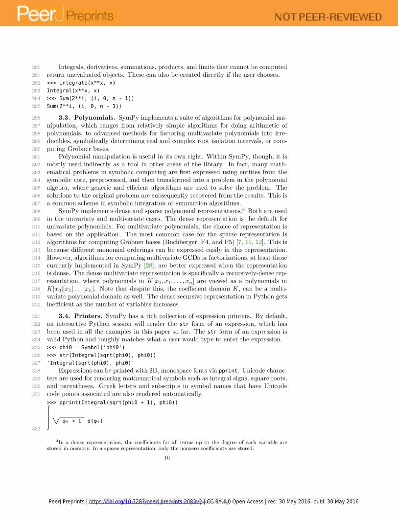
3.4. Printers. SymPy has a rich collection of expression printers. By default,321an interactive Python session will render the str form of an expression, which has322been used in all the examples in this paper so far. The str form of an expression is323valid Python and roughly matches what a user would type to enter the expression.324>>> phi0 = Symbol('phi0')325>>> str(Integral(sqrt(phi0), phi0))326'Integral(sqrt(phi0), phi0)'327

Expressions can be printed with 2D, monospace fonts via pprint. Unicode charac-328ters are used for rendering mathematical symbols such as integral signs, square roots,329and parentheses. Greek letters and subscripts in symbol names that have Unicode330code points associated are also rendered automatically.331>>> pprint(Integral(sqrt(phi0 + 1), phi0))⌠⎮ ________⎮ ╲╱ φ₀ + 1 d(φ₀)⌡

1

332

4In a dense representation, the coefficients for all terms up to the degree of each variable arestored in memory. In a sparse representation, only the nonzero coefficients are stored.

10


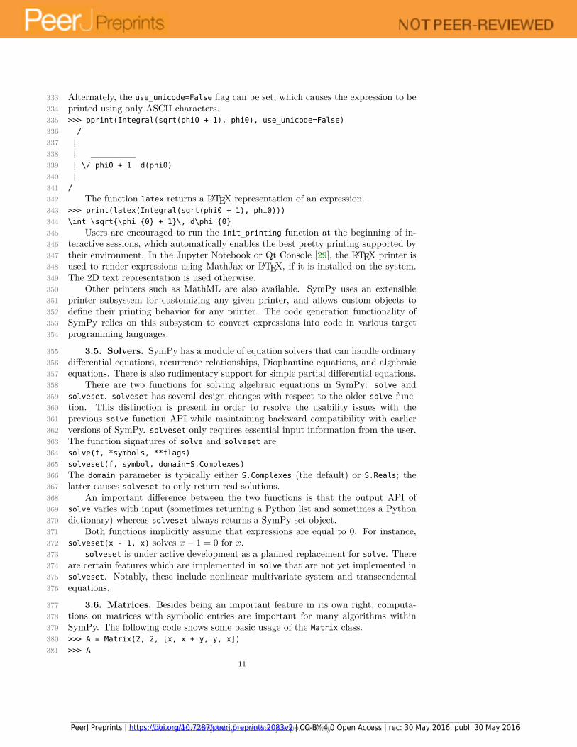
Alternately, the use_unicode=False flag can be set, which causes the expression to be333printed using only ASCII characters.334>>> pprint(Integral(sqrt(phi0 + 1), phi0), use_unicode=False)335

/336|337| __________338| \/ phi0 + 1 d(phi0)339|340

/341The function latex returns a LATEX representation of an expression.342

>>> print(latex(Integral(sqrt(phi0 + 1), phi0)))343\int \sqrt{\phi_{0} + 1}\, d\phi_{0}344

Users are encouraged to run the init_printing function at the beginning of in-345teractive sessions, which automatically enables the best pretty printing supported by346their environment. In the Jupyter Notebook or Qt Console [29], the LATEX printer is347used to render expressions using MathJax or LATEX, if it is installed on the system.348The 2D text representation is used otherwise.349

Other printers such as MathML are also available. SymPy uses an extensible350printer subsystem for customizing any given printer, and allows custom objects to351define their printing behavior for any printer. The code generation functionality of352SymPy relies on this subsystem to convert expressions into code in various target353programming languages.354

3.5. Solvers. SymPy has a module of equation solvers that can handle ordinary355differential equations, recurrence relationships, Diophantine equations, and algebraic356equations. There is also rudimentary support for simple partial differential equations.357

There are two functions for solving algebraic equations in SymPy: solve and358solveset. solveset has several design changes with respect to the older solve func-359tion. This distinction is present in order to resolve the usability issues with the360previous solve function API while maintaining backward compatibility with earlier361versions of SymPy. solveset only requires essential input information from the user.362The function signatures of solve and solveset are363solve(f, *symbols, **flags)364solveset(f, symbol, domain=S.Complexes)365The domain parameter is typically either S.Complexes (the default) or S.Reals; the366latter causes solveset to only return real solutions.367

An important difference between the two functions is that the output API of368solve varies with input (sometimes returning a Python list and sometimes a Python369dictionary) whereas solveset always returns a SymPy set object.370

Both functions implicitly assume that expressions are equal to 0. For instance,371solveset(x - 1, x) solves x− 1 = 0 for x.372

solveset is under active development as a planned replacement for solve. There373are certain features which are implemented in solve that are not yet implemented in374solveset. Notably, these include nonlinear multivariate system and transcendental375equations.376

3.6. Matrices. Besides being an important feature in its own right, computa-377tions on matrices with symbolic entries are important for many algorithms within378SymPy. The following code shows some basic usage of the Matrix class.379>>> A = Matrix(2, 2, [x, x + y, y, x])380>>> A381

11


Matrix([382[x, x + y],383[y, x]])384

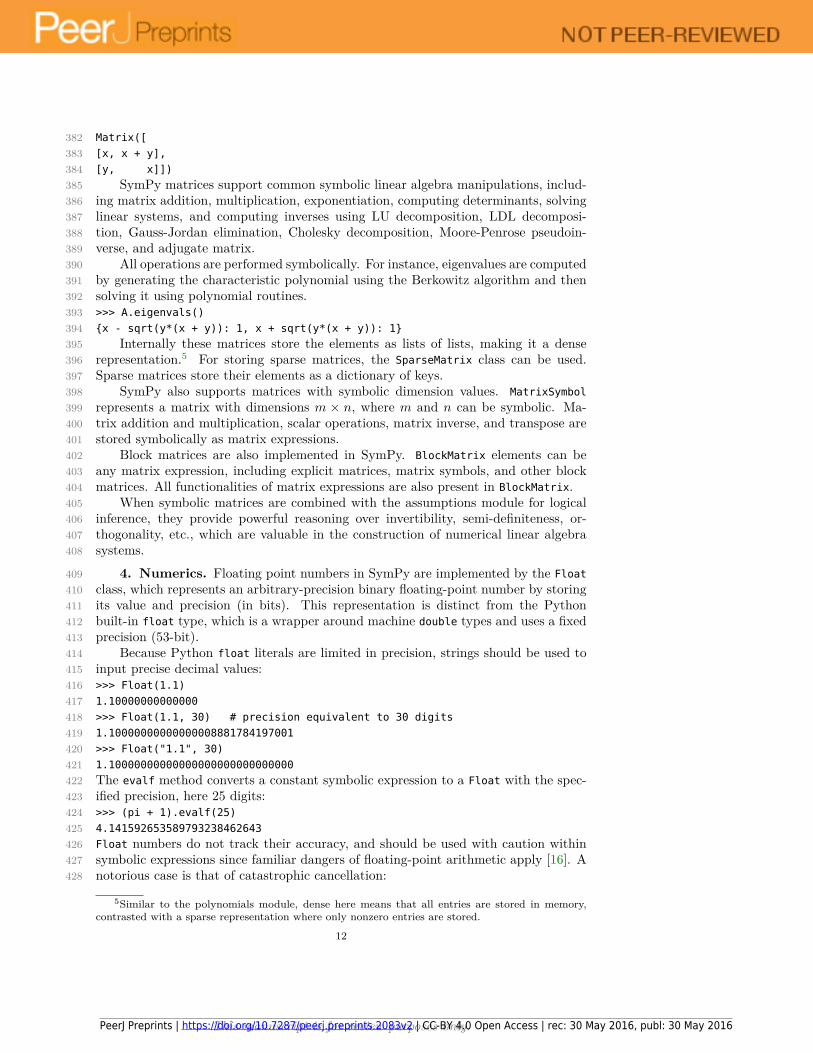
SymPy matrices support common symbolic linear algebra manipulations, includ-385ing matrix addition, multiplication, exponentiation, computing determinants, solving386linear systems, and computing inverses using LU decomposition, LDL decomposi-387tion, Gauss-Jordan elimination, Cholesky decomposition, Moore-Penrose pseudoin-388verse, and adjugate matrix.389

All operations are performed symbolically. For instance, eigenvalues are computed390by generating the characteristic polynomial using the Berkowitz algorithm and then391solving it using polynomial routines.392>>> A.eigenvals()393{x - sqrt(y*(x + y)): 1, x + sqrt(y*(x + y)): 1}394

Internally these matrices store the elements as lists of lists, making it a dense395representation.5 For storing sparse matrices, the SparseMatrix class can be used.396Sparse matrices store their elements as a dictionary of keys.397

SymPy also supports matrices with symbolic dimension values. MatrixSymbol398represents a matrix with dimensions m × n, where m and n can be symbolic. Ma-399trix addition and multiplication, scalar operations, matrix inverse, and transpose are400stored symbolically as matrix expressions.401

Block matrices are also implemented in SymPy. BlockMatrix elements can be402any matrix expression, including explicit matrices, matrix symbols, and other block403matrices. All functionalities of matrix expressions are also present in BlockMatrix.404

When symbolic matrices are combined with the assumptions module for logical405inference, they provide powerful reasoning over invertibility, semi-definiteness, or-406thogonality, etc., which are valuable in the construction of numerical linear algebra407systems.408

4. Numerics. Floating point numbers in SymPy are implemented by the Float409class, which represents an arbitrary-precision binary floating-point number by storing410its value and precision (in bits). This representation is distinct from the Python411built-in float type, which is a wrapper around machine double types and uses a fixed412precision (53-bit).413

Because Python float literals are limited in precision, strings should be used to414input precise decimal values:415>>> Float(1.1)4161.10000000000000417>>> Float(1.1, 30) # precision equivalent to 30 digits4181.10000000000000008881784197001419>>> Float("1.1", 30)4201.10000000000000000000000000000421The evalf method converts a constant symbolic expression to a Float with the spec-422ified precision, here 25 digits:423>>> (pi + 1).evalf(25)4244.141592653589793238462643425Float numbers do not track their accuracy, and should be used with caution within426symbolic expressions since familiar dangers of floating-point arithmetic apply [16]. A427notorious case is that of catastrophic cancellation:428

5Similar to the polynomials module, dense here means that all entries are stored in memory,contrasted with a sparse representation where only nonzero entries are stored.

12


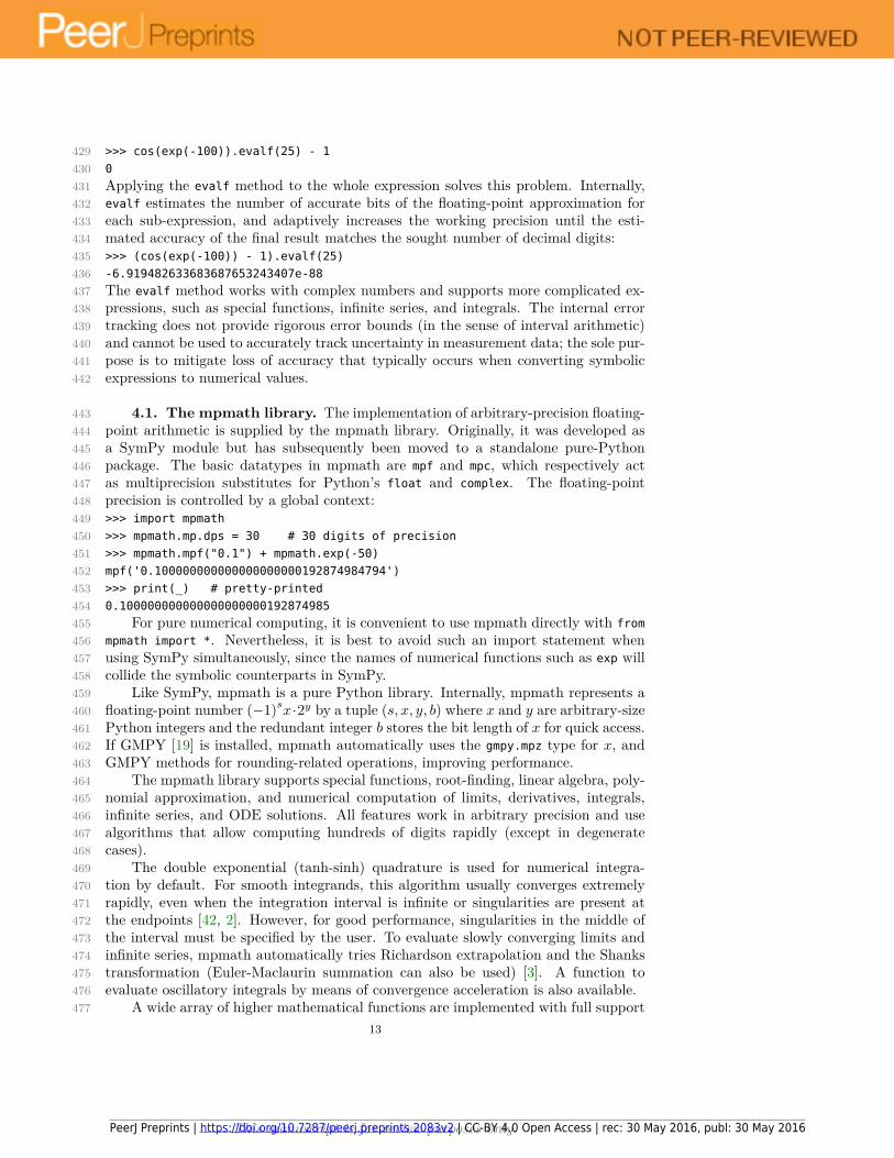
>>> cos(exp(-100)).evalf(25) - 14290430Applying the evalf method to the whole expression solves this problem. Internally,431evalf estimates the number of accurate bits of the floating-point approximation for432each sub-expression, and adaptively increases the working precision until the esti-433mated accuracy of the final result matches the sought number of decimal digits:434>>> (cos(exp(-100)) - 1).evalf(25)435-6.919482633683687653243407e-88436The evalf method works with complex numbers and supports more complicated ex-437pressions, such as special functions, infinite series, and integrals. The internal error438tracking does not provide rigorous error bounds (in the sense of interval arithmetic)439and cannot be used to accurately track uncertainty in measurement data; the sole pur-440pose is to mitigate loss of accuracy that typically occurs when converting symbolic441expressions to numerical values.442

4.1. The mpmath library. The implementation of arbitrary-precision floating-443point arithmetic is supplied by the mpmath library. Originally, it was developed as444a SymPy module but has subsequently been moved to a standalone pure-Python445package. The basic datatypes in mpmath are mpf and mpc, which respectively act446as multiprecision substitutes for Python’s float and complex. The floating-point447precision is controlled by a global context:448>>> import mpmath449>>> mpmath.mp.dps = 30 # 30 digits of precision450>>> mpmath.mpf("0.1") + mpmath.exp(-50)451mpf('0.100000000000000000000192874984794')452>>> print(_) # pretty-printed4530.100000000000000000000192874985454

For pure numerical computing, it is convenient to use mpmath directly with from455mpmath import *. Nevertheless, it is best to avoid such an import statement when456using SymPy simultaneously, since the names of numerical functions such as exp will457collide the symbolic counterparts in SymPy.458

Like SymPy, mpmath is a pure Python library. Internally, mpmath represents a459floating-point number (−1)sx·2y by a tuple (s, x, y, b) where x and y are arbitrary-size460Python integers and the redundant integer b stores the bit length of x for quick access.461If GMPY [19] is installed, mpmath automatically uses the gmpy.mpz type for x, and462GMPY methods for rounding-related operations, improving performance.463

The mpmath library supports special functions, root-finding, linear algebra, poly-464nomial approximation, and numerical computation of limits, derivatives, integrals,465infinite series, and ODE solutions. All features work in arbitrary precision and use466algorithms that allow computing hundreds of digits rapidly (except in degenerate467cases).468

The double exponential (tanh-sinh) quadrature is used for numerical integra-469tion by default. For smooth integrands, this algorithm usually converges extremely470rapidly, even when the integration interval is infinite or singularities are present at471the endpoints [42, 2]. However, for good performance, singularities in the middle of472the interval must be specified by the user. To evaluate slowly converging limits and473infinite series, mpmath automatically tries Richardson extrapolation and the Shanks474transformation (Euler-Maclaurin summation can also be used) [3]. A function to475evaluate oscillatory integrals by means of convergence acceleration is also available.476

A wide array of higher mathematical functions are implemented with full support477

13


for complex values of all parameters and arguments, including complete and incom-478plete gamma functions, Bessel functions, orthogonal polynomials, elliptic functions479and integrals, zeta and polylogarithm functions, the generalized hypergeometric func-480tion, and the Meijer G-function. The Meijer G-function instance G3,0

1,3(0; 1

2 ,−1,− 32 |x)

481is a good test case [43]; past versions of both Maple and Mathematica produced in-482correct numerical values for large x > 0. Here, mpmath automatically removes an483internal singularity and compensates for cancellations (amounting to 656 bits of pre-484cision when x = 10000), giving correct values:485>>> mpmath.mp.dps = 15486>>> mpmath.meijerg([[],[0]],[[-0.5,-1,-1.5],[]],10000)487mpf('2.4392576907199564e-94')488

Equivalently, with SymPy’s interface this function can be evaluated as:489>>> meijerg([[],[0]],[[-S(1)/2,-1,-S(3)/2],[]],10000).evalf()4902.43925769071996e-94491

Symbolic integration and summation often produces hypergeometric and Meijer492G-function closed forms (see Subsection 3.2); numerical evaluation of such special493functions is a useful complement to direct numerical integration and summation.494

5. Domain Specific Submodules. SymPy includes several packages that al-495low users to solve domain specific problems. For example, a comprehensive physics496package is included that is useful for solving problems in mechanics, optics, and quan-497tum mechanics along with support for manipulating physical quantities with units.498

5.1. Classical Mechanics. One of the core domains that SymPy suports is the499physics of classical mechanics. This is in turn separated into two distinct components:500vector algebra symbolics and mechanics.501

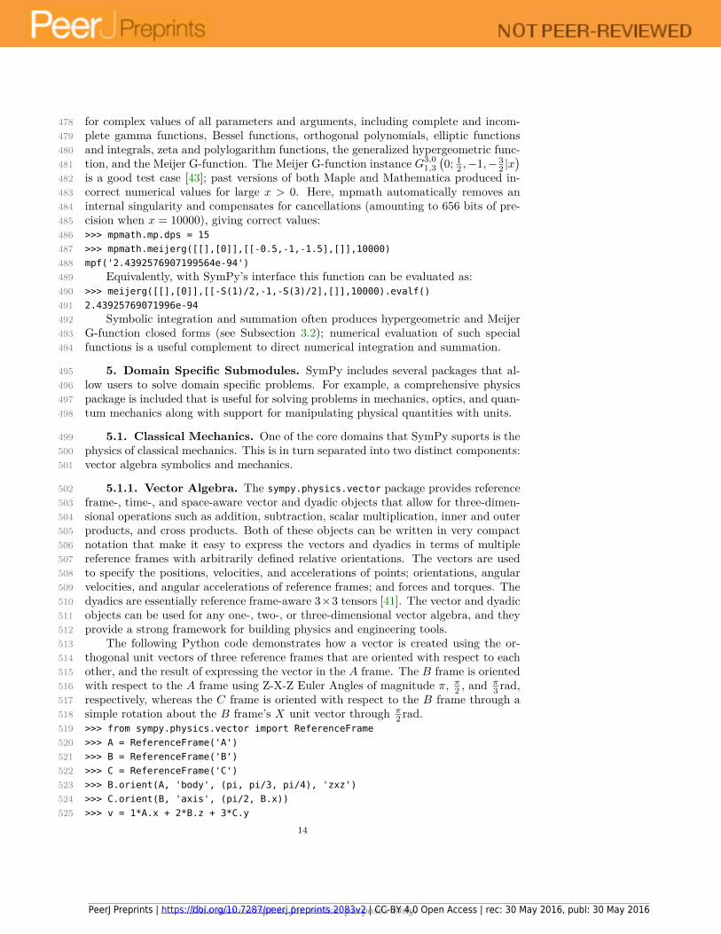
5.1.1. Vector Algebra. The sympy.physics.vector package provides reference502frame-, time-, and space-aware vector and dyadic objects that allow for three-dimen-503sional operations such as addition, subtraction, scalar multiplication, inner and outer504products, and cross products. Both of these objects can be written in very compact505notation that make it easy to express the vectors and dyadics in terms of multiple506reference frames with arbitrarily defined relative orientations. The vectors are used507to specify the positions, velocities, and accelerations of points; orientations, angular508velocities, and angular accelerations of reference frames; and forces and torques. The509dyadics are essentially reference frame-aware 3×3 tensors [41]. The vector and dyadic510objects can be used for any one-, two-, or three-dimensional vector algebra, and they511provide a strong framework for building physics and engineering tools.512

The following Python code demonstrates how a vector is created using the or-513thogonal unit vectors of three reference frames that are oriented with respect to each514other, and the result of expressing the vector in the A frame. The B frame is oriented515with respect to the A frame using Z-X-Z Euler Angles of magnitude π, π2 , and

π3 rad,516

respectively, whereas the C frame is oriented with respect to the B frame through a517simple rotation about the B frame’s X unit vector through π

2 rad.518>>> from sympy.physics.vector import ReferenceFrame519>>> A = ReferenceFrame('A')520>>> B = ReferenceFrame('B')521>>> C = ReferenceFrame('C')522>>> B.orient(A, 'body', (pi, pi/3, pi/4), 'zxz')523>>> C.orient(B, 'axis', (pi/2, B.x))524>>> v = 1*A.x + 2*B.z + 3*C.y525

14


>>> v526A.x + 2*B.z + 3*C.y527>>> v.express(A)528A.x + 5*sqrt(3)/2*A.y + 5/2*A.z529

5.1.2. Mechanics. The sympy.physics.mechanics package utilizes the sympy.530physics.vector package to populate time-aware particle and rigid-body objects to531fully describe the kinematics and kinetics of a rigid multi-body system. These objects532store all of the information needed to derive the ordinary differential or differential533algebraic equations that govern the motion of the system, i.e., the equations of mo-534tion. These equations of motion abide by Newton’s laws of motion and can handle535arbitrary kinematic constraints or complex loads. The package offers two automated536methods for formulating the equations of motion based on Lagrangian Dynamics [22]537and Kane’s Method [21]. Lastly, there are automated linearization routines for con-538strained dynamical systems [30].539

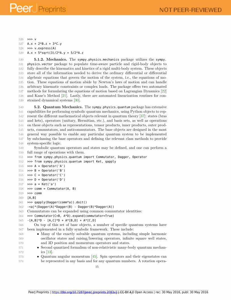
5.2. Quantum Mechanics. The sympy.physics.quantum package has extensive540capabilities for performing symbolic quantum mechanics, using Python objects to rep-541resent the different mathematical objects relevant in quantum theory [37]: states (bras542and kets), operators (unitary, Hermitian, etc.), and basis sets, as well as operations543on these objects such as representations, tensor products, inner products, outer prod-544ucts, commutators, and anticommutators. The base objects are designed in the most545general way possible to enable any particular quantum system to be implemented546by subclassing the base operators and defining the relevant class methods to provide547system-specific logic.548

Symbolic quantum operators and states may be defined, and one can perform a549full range of operations with them.550>>> from sympy.physics.quantum import Commutator, Dagger, Operator551>>> from sympy.physics.quantum import Ket, qapply552>>> A = Operator('A')553>>> B = Operator('B')554>>> C = Operator('C')555>>> D = Operator('D')556>>> a = Ket('a')557>>> comm = Commutator(A, B)558>>> comm559[A,B]560>>> qapply(Dagger(comm*a)).doit()561-<a|*(Dagger(A)*Dagger(B) - Dagger(B)*Dagger(A))562Commutators can be expanded using common commutator identities:563>>> Commutator(C+B, A*D).expand(commutator=True)564-[A,B]*D - [A,C]*D + A*[B,D] + A*[C,D]565

On top of this set of base objects, a number of specific quantum systems have566been implemented in a fully symbolic framework. These include:567

• Many of the exactly solvable quantum systems, including simple harmonic568oscillator states and raising/lowering operators, infinite square well states,569and 3D position and momentum operators and states.570

• Second quantized formalism of non-relativistic many-body quantum mechan-571ics [13].572

• Quantum angular momentum [45]. Spin operators and their eigenstates can573be represented in any basis and for any quantum numbers. A rotation opera-574

15


tor representing the Wigner-D matrix, which may be defined symbolically or575numerically, is also implemented to rotate spin eigenstates. Functionality for576coupling and uncoupling of arbitrary spin eigenstates is provided, including577symbolic representations of Clebsch-Gordon coefficients and Wigner symbols.578

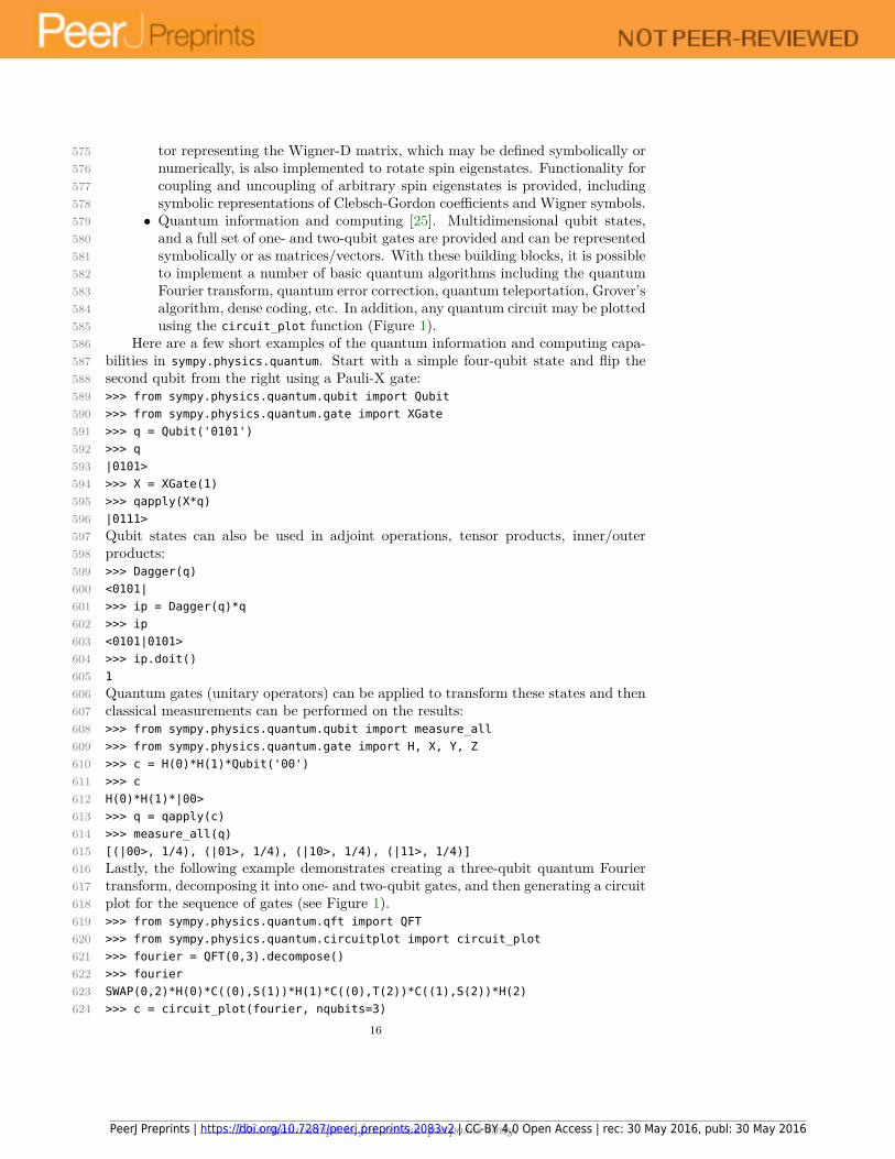
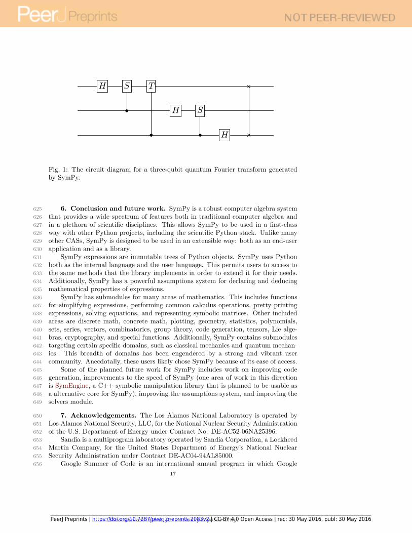
• Quantum information and computing [25]. Multidimensional qubit states,579and a full set of one- and two-qubit gates are provided and can be represented580symbolically or as matrices/vectors. With these building blocks, it is possible581to implement a number of basic quantum algorithms including the quantum582Fourier transform, quantum error correction, quantum teleportation, Grover’s583algorithm, dense coding, etc. In addition, any quantum circuit may be plotted584using the circuit_plot function (Figure 1).585

Here are a few short examples of the quantum information and computing capa-586bilities in sympy.physics.quantum. Start with a simple four-qubit state and flip the587second qubit from the right using a Pauli-X gate:588>>> from sympy.physics.quantum.qubit import Qubit589>>> from sympy.physics.quantum.gate import XGate590>>> q = Qubit('0101')591>>> q592|0101>593>>> X = XGate(1)594>>> qapply(X*q)595|0111>596Qubit states can also be used in adjoint operations, tensor products, inner/outer597products:598>>> Dagger(q)599<0101|600>>> ip = Dagger(q)*q601>>> ip602<0101|0101>603>>> ip.doit()6041605Quantum gates (unitary operators) can be applied to transform these states and then606classical measurements can be performed on the results:607>>> from sympy.physics.quantum.qubit import measure_all608>>> from sympy.physics.quantum.gate import H, X, Y, Z609>>> c = H(0)*H(1)*Qubit('00')610>>> c611H(0)*H(1)*|00>612>>> q = qapply(c)613>>> measure_all(q)614[(|00>, 1/4), (|01>, 1/4), (|10>, 1/4), (|11>, 1/4)]615Lastly, the following example demonstrates creating a three-qubit quantum Fourier616transform, decomposing it into one- and two-qubit gates, and then generating a circuit617plot for the sequence of gates (see Figure 1).618>>> from sympy.physics.quantum.qft import QFT619>>> from sympy.physics.quantum.circuitplot import circuit_plot620>>> fourier = QFT(0,3).decompose()621>>> fourier622SWAP(0,2)*H(0)*C((0),S(1))*H(1)*C((0),T(2))*C((1),S(2))*H(2)623>>> c = circuit_plot(fourier, nqubits=3)624

16


H S T

H S

H

Fig. 1: The circuit diagram for a three-qubit quantum Fourier transform generatedby SymPy.

6. Conclusion and future work. SymPy is a robust computer algebra system625that provides a wide spectrum of features both in traditional computer algebra and626in a plethora of scientific disciplines. This allows SymPy to be used in a first-class627way with other Python projects, including the scientific Python stack. Unlike many628other CASs, SymPy is designed to be used in an extensible way: both as an end-user629application and as a library.630

SymPy expressions are immutable trees of Python objects. SymPy uses Python631both as the internal language and the user language. This permits users to access to632the same methods that the library implements in order to extend it for their needs.633Additionally, SymPy has a powerful assumptions system for declaring and deducing634mathematical properties of expressions.635

SymPy has submodules for many areas of mathematics. This includes functions636for simplifying expressions, performing common calculus operations, pretty printing637expressions, solving equations, and representing symbolic matrices. Other included638areas are discrete math, concrete math, plotting, geometry, statistics, polynomials,639sets, series, vectors, combinatorics, group theory, code generation, tensors, Lie alge-640bras, cryptography, and special functions. Additionally, SymPy contains submodules641targeting certain specific domains, such as classical mechanics and quantum mechan-642ics. This breadth of domains has been engendered by a strong and vibrant user643community. Anecdotally, these users likely chose SymPy because of its ease of access.644

Some of the planned future work for SymPy includes work on improving code645generation, improvements to the speed of SymPy (one area of work in this direction646is SymEngine, a C++ symbolic manipulation library that is planned to be usable as647a alternative core for SymPy), improving the assumptions system, and improving the648solvers module.649

7. Acknowledgements. The Los Alamos National Laboratory is operated by650Los Alamos National Security, LLC, for the National Nuclear Security Administration651of the U.S. Department of Energy under Contract No. DE-AC52-06NA25396.652

Sandia is a multiprogram laboratory operated by Sandia Corporation, a Lockheed653Martin Company, for the United States Department of Energy’s National Nuclear654Security Administration under Contract DE-AC04-94AL85000.655

Google Summer of Code is an international annual program in which Google656

17


https://github.com/symengine/symengine

awards stipends to all students who successfully complete a requested free and open-657source software coding project during the summer.658

The author of this paper Francesco Bonazzi thanks the Deutsche Forschungsge-659meinschaft (DFG) for its financial support via the International Research Training660Group 1524 "Self-Assembled Soft Matter Nano-Structures at Interfaces."661

8. References.662REFERENCES663

[1] W. W. Adams and P. Loustaunau, An introduction to Gröbner bases, no. 3, American Math-664ematical Society, 1994.665

[2] D. H. Bailey, K. Jeyabalan, and X. S. Li, A comparison of three high-precision quadrature666schemes, Experimental Mathematics, 14 (2005), pp. 317–329.667

[3] C. M. Bender and S. A. Orszag, Advanced Mathematical Methods for Scientists and Engi-668neers, Springer, 1st ed., October 1999.669

[4] N. Biggs, E. K. Lloyd, and R. J. Wilson, Graph Theory, 1736-1936, Oxford University670Press, 1976.671

[5] M. Bronstein, Poor Man’s Integrator, http://www-sop.inria.fr/cafe/Manuel.Bronstein/pmint.672[6] M. Bronstein, Symbolic Integration I: Transcendental Functions, Springer–Verlag, New York,673

NY, USA, 2005.674[7] B. Buchberger, Ein Algorithmus zum Auffinden der Basis Elemente des Restklassenrings675

nach einem nulldimensionalen Polynomideal, PhD thesis, University of Innsbruck, Inns-676bruck, Austria, 1965.677

[8] J. Carette, Understanding Expression Simplification, in ISSAC ’04: Proceedings of the6782004 International Symposium on Symbolic and Algebraic Computation, New York,679NY, USA, 2004, ACM Press, pp. 72–79, http://dx.doi.org/http://doi.acm.org/10.1145/6801005285.1005298.681

[9] D. Cervone, Mathjax: a platform for mathematics on the web, Notices of the AMS, 59 (2012),682pp. 312–316.683

[10] R. Cimrman, SfePy - write your own FE application, in Proceedings of the 6th European684Conference on Python in Science (EuroSciPy 2013), P. de Buyl and N. Varoquaux, eds.,6852014, pp. 65–70. http://arxiv.org/abs/1404.6391.686

[11] J. C. Faugère, A New Efficient Algorithm for Computing Gröbner Bases (F4), Journal of687Pure and Applied Algebra, 139 (1999), pp. 61–88, http://www-calfor.lip6.fr/~jcf/Papers/688F99a.pdf.689

[12] J. C. Faugère, A New Efficient Algorithm for Computing Gröbner Bases Without Reduc-690tion To Zero (F5), in ISSAC ’02: Proceedings of the 2002 International Symposium on691Symbolic and Algebraic Computation, New York, NY, USA, 2002, ACM Press, pp. 75–69283, http://dx.doi.org/http://doi.acm.org/10.1145/780506.780516, http://www-calfor.lip6.693fr/~jcf/Papers/F02a.pdf.694

[13] A. Fetter and J. Walecka, Quantum Theory of Many-Particle Systems, Dover Publications,6952003.696

[14] H. Fu, X. Zhong, and Z. Zeng, Automated and Readable Simplification of Trigonometric697Expressions, Mathematical and Computer Modelling, 55 (2006), pp. 1169–1177.698

[15] G. Gede, D. L. Peterson, A. S. Nanjangud, J. K. Moore, and M. Hubbard, Constrained699multibody dynamics with Python: From symbolic equation generation to publication, in700ASME 2013 International Design Engineering Technical Conferences and Computers and701Information in Engineering Conference, American Society of Mechanical Engineers, 2013,702pp. V07BT10A051–V07BT10A051.703

[16] D. Goldberg, What every computer scientist should know about floating-point arithmetic,704ACM Computing Surveys (CSUR), 23 (1991), pp. 5–48.705

[17] R. W. Gosper, Decision procedure for indefinite hypergeometric summation, Proceedings of706the National Academy of Sciences, 75 (1978), pp. 40–42.707

[18] D. Gruntz, On Computing Limits in a Symbolic Manipulation System, PhD thesis, Swiss708Federal Institute of Technology, Zürich, Switzerland, 1996.709

[19] C. V. Horsen, GMPY. https://pypi.python.org/pypi/gmpy2, 2015.710[20] J. D. Hunter, Matplotlib: A 2d graphics environment, Computing In Science & Engineering,711

9 (2007), pp. 90–95.712[21] T. R. Kane and D. A. Levinson, Dynamics, Theory and Applications, McGraw Hill, 1985.713[22] J. Lagrange, Mécanique analytique, no. v. 1 in Mécanique analytique, Ve Courcier, 1811.714

18


http://www-sop.inria.fr/cafe/Manuel.Bronstein/pmint

http://dx.doi.org/http://doi.acm.org/10.1145/1005285.1005298



http://www-calfor.lip6.fr/~jcf/Papers/F99a.pdf







https://pypi.python.org/pypi/gmpy2

[23] S. Lang, Introduction to transcendental numbers, Reading, Mass, (1966).715[24] M. Lutz, Learning Python, O’Reilly Media, Inc., 2013.716[25] M. Nielsen and I. Chuang, Quantum Computation and Quantum Information, Cambridge717

University Press, 2011.718[26] A. Nijenhuis and H. S. Wilf, Combinatorial Algorithms: For Computers and Calculators,719

Academic Press, New York, NY, USA, second ed., 1978.720[27] T. E. Oliphant, Python for scientific computing, Computing in Science & Engineering, 9721

(2007), pp. 10–20.722[28] M. Paprocki, Design and implementation issues of a computer algebra system in an inter-723

preted, dynamically typed programming language, master’s thesis, University of Technology724of Wrocław, Poland, 2010.725

[29] F. Pérez and B. E. Granger, IPython: a system for interactive scientific computing, Com-726puting in Science & Engineering, 9 (2007), pp. 21–29.727

[30] D. L. Peterson, G. Gede, and M. Hubbard, Symbolic linearization of equations of motion728of constrained multibody systems, Multibody System Dynamics, 33 (2014), pp. 143–161,729http://dx.doi.org/10.1007/s11044-014-9436-5.730

[31] M. Petkovšek, H. S. Wilf, and D. Zeilberger, A= BAK peters, Wellesley, MA, (1996).731[32] E. Raymond, The cathedral and the bazaar, Knowledge, Technology & Policy, 12 (1999), pp. 23–732

49.733[33] K. Roach, Hypergeometric function representations, in ISSAC ’96: Proceedings of the 1996734

International Symposium on Symbolic and Algebraic Computation, New York, NY, USA,7351996, ACM Press, pp. 301–308, http://dx.doi.org/http://doi.acm.org/10.1145/236869.736237088, http://www.planetquantum.com/TheMission/Papers/Issac96.pdf.737

[34] K. Roach, Meijer G function representations, in ISSAC ’97: Proceedings of the 1997 inter-738national symposium on Symbolic and algebraic computation, New York, NY, USA, 1997,739ACM, pp. 205–211, http://dx.doi.org/http://doi.acm.org/10.1145/258726.258784.740

[35] M. Rocklin and A. R. Terrel, Symbolic statistics with SymPy, Computing in Science and741Engineering, 14 (2012), http://dx.doi.org/10.1109/MCSE.2012.56.742

[36] L. Rosen, Open source licensing, vol. 692, Prentice Hall, 2005.743[37] J. Sakurai and J. Napolitano, Modern Quantum Mechanics, Addison-Wesley, 2010.744[38] M. Shaw and D. Garlan, Software Architecture: Perspectives on an Emerging Discipline,745

Prentice Hall, 1996. Prentice Hall Ordering Information.746[39] W. Stein and D. Joyner, SAGE: System for Algebra and Geometry Experimentation, Com-747

munications in Computer Algebra, 39 (2005).748[40] G. J. Sussman and J. Wisdom, Functional Differential Geometry, Massachusetts Institute of749

Technology Press, 2013.750[41] C.-T. Tai, Generalized vector and dyadic analysis: applied mathematics in field theory, vol. 9,751

Wiley-IEEE Press, 1997.752[42] H. Takahasi and M. Mori, Double exponential formulas for numerical integration, Publica-753

tions of the Research Institute for Mathematical Sciences, 9 (1974), pp. 721–741.754[43] V. T. Toth, Maple and Meijer’s G-function: a numerical instability and a cure. http://www.755

vttoth.com/CMS/index.php/technical-notes/67, 2007.756[44] M. J. Turk, B. D. Smith, J. S. Oishi, S. Skory, S. W. Skillman, T. Abel, and M. L.757

Norman, yt: A Multi-code Analysis Toolkit for Astrophysical Simulation Data, The As-758trophysical Journal Supplement Series, 192 (2011), pp. 9–+, http://dx.doi.org/10.1088/7590067-0049/192/1/9, arXiv:1011.3514.760

[45] R. Zare, Angular Momentum: Understanding Spatial Aspects in Chemistry and Physics, Wi-761ley, 1991.762

19


http://dx.doi.org/10.1007/s11044-014-9436-5




http://www.planetquantum.com/TheMission/Papers/Issac96.pdf


http://dx.doi.org/10.1109/MCSE.2012.56

http://www.vttoth.com/CMS/index.php/technical-notes/67



http://dx.doi.org/10.1088/0067-0049/192/1/9

http://dx.doi.org/10.1088/0067-0049/192/1/9

http://dx.doi.org/10.1088/0067-0049/192/1/9

http://arxiv.org/abs/1011.3514

Documents

SYMPY:SYMBOLICCOMPUTINGINPYTHON 2 AARON MEURER 1. … · 2017-08-07 · 1 sympy:symboliccomputinginpython 2 aaron meurer∗, christopher p. smith†, mateusz paprocki‡, ondŘej