Embed Size (px)
Citation preview

Ondas viajeras singulares en ecuaciones nolineales de reacción-difusión
J. Calvo, J. Campos, V. Caselles, P. Guerrero, O. Sánchez,J. Soler
Dept. de Tecnologies de la Informació i les ComunicacionsUniversitat Pompeu Fabra.
Congreso de jóvenes investigadores16-20 Septiembre 2013, Sevilla
J. Calvo et al. Non-linear diffusion and traveling waves

Classical traveling waves
Its is widely known that the model
ut = νuxx + k u(1− u)
displays classical traveling waves u(t , x) = u(x − σt) forwavespeeds σ ≥ 2
√kν. (Fisher; Kolmogoroff, Petrovsky, Piscounoff, 1937)
13.2 Fisher–Kolmogoroff Equation 441
U !! + cU ! + U(1 " U) = 0, (13.8)
where primes denote differentiation with respect to z. A typical wavefront solution iswhere U at one end, say, as z # "$, is at one steady state and as z # $ it is at theother. So here we have an eigenvalue problem to determine the value, or values, of csuch that a nonnegative solution U of (13.8) exists which satisfies
limz#$ U(z) = 0, lim
z#"$U(z) = 1. (13.9)
At this stage we do not address the problem of how such a travelling wave solutionmight evolve from the partial differential equation (13.6) with given initial conditionsu(x, 0); we come back to this point later.
We study (13.8) for U in the (U, V ) phase plane where
U ! = V, V ! = "cV " U(1 " U), (13.10)
which gives the phase plane trajectories as solutions of
dVdU
= "cV " U(1 " U)
V. (13.11)
This has two singular points for (U, V ), namely, (0, 0) and (1, 0): these are the steadystates of course. A linear stability analysis (see Appendix A) shows that the eigenvalues! for the singular points are
(0, 0) : !± = 12
!"c ± (c2 " 4)1/2
"%
#stable node if c2 > 4stable spiral if c2 < 4
(1, 0) : !± = 12
!"c ± (c2 + 4)1/2
"% saddle point.
(13.12)
Figure 13.1(a) illustrates the phase plane trajectories.If c & cmin = 2 we see from (13.12) that the origin is a stable node, the case when
c = cmin giving a degenerate node. If c2 < 4 it is a stable spiral; that is, in the vicinity
Figure 13.1. (a) Phase plane trajectories for equation (13.8) for the travelling wavefront solution: here c2 >
4. (b) Travelling wavefront solution for the Fisher–Kolmogoroff equation (13.6): the wave velocity c & 2.(Murray, Mathematical Biology)
The corresponding profiles are monotone. These solutions aresupported in the whole line (as a subsidiary effect, informationis propagated instantaneously).
J. Calvo et al. Non-linear diffusion and traveling waves

Finite speed of propagation
Exponential tails can compromise some applications of thismodel. Can we fix that?
This would amount to use a diffusion term with the property offinite speed of propagation.
We will consider the following:the porous media equationflux saturation: the “relativistic heat equation”.
J. Calvo et al. Non-linear diffusion and traveling waves

Traveling waves for the porous media equation
The porous media equation (density-dependent diffusion):
ut = ν(um−1ux)x , m > 1.
Finite propagation speed.The heat equation is recovered for m = 1.
J. Calvo et al. Non-linear diffusion and traveling waves

Traveling waves for the porous media equation
The following model admits traveling wave solutions:
ut = ν(um−1ux)x + k u(1− u).
(Newman, J. Theor. Biol. 1980)
13.4 Density-Dependent Diffusion-Reaction Diffusion Models 453
Figure 13.4. Qualitative phase plane trajectories for the travelling wave equations (13.52) for various c.(After Aronson 1980) In (a) no trajectory is possible from (1, 0) to U = 0 at a finite V . In (b) and (c) travellingwave solutions from U = 1 to U = 0 are possible but with different characteristics: the travelling wavesolutions in (d) illustrate these differences. Importantly the solution corresponding to (b) has a discontinuousderivative at the leading edge.
(U, V ) = (0, 0), (1, 0), (0,!c).
A linear analysis about (1, 0) and (0,!c) shows them to be saddle points while (0, 0)
is like a stable nonlinear node—nonlinear because of the U V in the U -equation in(13.52). Figure 13.4 illustrates the phase trajectories for (13.52) for various c. FromSection 11.2 we can expect the possibility of a wave with a discontinuous tangent at aspecific point zc, the one where U " 0 for z # zc. This corresponds to a phase trajectorywhich goes from (1, 0) to a point on the U = 0 axis at some finite nonzero negativeV . Referring now to Figure 13.4(a), if 0 < c < cmin there is no trajectory possiblefrom (1, 0) to U = 0 except unrealistically for infinite V . As c increases there is abifurcation value cmin for which there is a unique trajectory from (1, 0) to (0,!cmin)
as shown in Figure 13.4(b). This means that at the wavefront zc, where U = 0, there isa discontinuity in the derivative from V = U $ = !cmin to U $ = 0 and U = 0 for allz > zc; see Figure 13.4(d). As c increases beyond cmin a trajectory always exists from(1, 0) to (0, 0) but now the wave solution has U % 0 and U $ % 0 as z % &; this typeof wave is also illustrated in Figure 13.4(d).
As regards the exact solution, the trajectory connecting (1, 0) to (0,!c) in Fig-ure 13.4(b) is in fact a straight line V = !cmin(1 ! U) if cmin is appropriately chosen.In other words this is a solution of the phase plane equation which, from (13.51), is
dVdU
= !cV ! V 2 ! U(1 ! U)
U V.
Substitution of V = !cmin(1 ! U) in this equation, with c = cmin, shows that cmin =1/
'2. If we now return to the first of the phase equations in (13.51), namely, U $ = V
and use the phase trajectory solution V = !(1 ! U)/'
2 we get
U $ = !1 ! U'2
,
(Murray, Mathematical Biology)
J. Calvo et al. Non-linear diffusion and traveling waves
The “relativistic heat equation”: a numerical illustration
classical heat eq.relativistic heat eq.
t = 0.075
10.80.60.40.20
2
1.5
1
0.5
0
(Andreu, Calvo, Mazón, Soler, Verbeni, Math. Mod. Meth. Appl. Sci. 2011)
J. Calvo et al. Non-linear diffusion and traveling waves

The “relativistic heat equation”: a numerical illustration
classical heat eq.relativistic heat eq.
t = 0.15
10.80.60.40.20
2
1.5
1
0.5
0
(Andreu, Calvo, Mazón, Soler, Verbeni, Math. Mod. Meth. Appl. Sci. 2011)
J. Calvo et al. Non-linear diffusion and traveling waves

The “relativistic heat equation”: a numerical illustration
classical heat eq.relativistic heat eq.
t = 0.3
10.80.60.40.20
2
1.5
1
0.5
0
(Andreu, Calvo, Mazón, Soler, Verbeni, Math. Mod. Meth. Appl. Sci. 2011)
J. Calvo et al. Non-linear diffusion and traveling waves
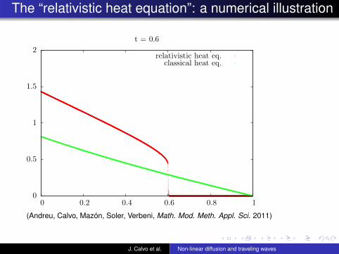
The “relativistic heat equation”: a numerical illustration
classical heat eq.relativistic heat eq.
t = 0.6
10.80.60.40.20
2
1.5
1
0.5
0
(Andreu, Calvo, Mazón, Soler, Verbeni, Math. Mod. Meth. Appl. Sci. 2011)
J. Calvo et al. Non-linear diffusion and traveling waves

The “relativistic heat equation”: a numerical illustration
classical heat eq.relativistic heat eq.
t = 0.9
10.80.60.40.20
2
1.5
1
0.5
0
(Andreu, Calvo, Mazón, Soler, Verbeni, Math. Mod. Meth. Appl. Sci. 2011)
J. Calvo et al. Non-linear diffusion and traveling waves
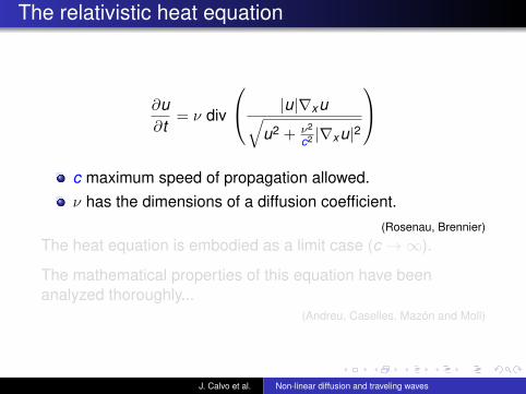
The relativistic heat equation
∂u∂t
= ν div
|u|∇xu√u2 + ν2
c2 |∇xu|2
c maximum speed of propagation allowed.ν has the dimensions of a diffusion coefficient.
(Rosenau, Brennier)
The heat equation is embodied as a limit case (c →∞).
The mathematical properties of this equation have beenanalyzed thoroughly...
(Andreu, Caselles, Mazón and Moll)
J. Calvo et al. Non-linear diffusion and traveling waves
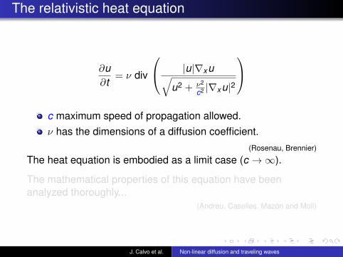
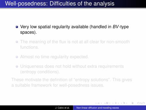
Well-posedness: Difficulties of the analysis
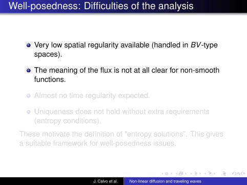
Very low spatial regularity available (handled in BV -typespaces).
The meaning of the flux is not at all clear for non-smoothfunctions.
Almost no time regularity expected.
Uniqueness does not hold without extra requirements(entropy conditions).
These motivate the definition of “entropy solutions”. This givesa suitable framework for well-posedness issues.
J. Calvo et al. Non-linear diffusion and traveling waves
Well-posedness: Difficulties of the analysis
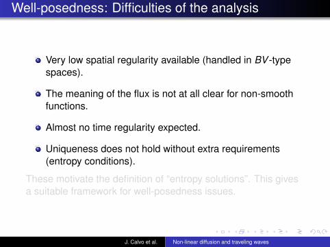
Very low spatial regularity available (handled in BV -typespaces).
The meaning of the flux is not at all clear for non-smoothfunctions.
Almost no time regularity expected.
Uniqueness does not hold without extra requirements(entropy conditions).
These motivate the definition of “entropy solutions”. This givesa suitable framework for well-posedness issues.
J. Calvo et al. Non-linear diffusion and traveling waves

Well-posedness: Difficulties of the analysis
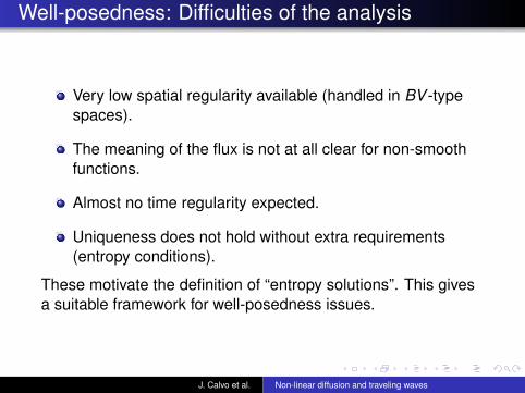
Very low spatial regularity available (handled in BV -typespaces).
The meaning of the flux is not at all clear for non-smoothfunctions.
Almost no time regularity expected.
Uniqueness does not hold without extra requirements(entropy conditions).
These motivate the definition of “entropy solutions”. This givesa suitable framework for well-posedness issues.
J. Calvo et al. Non-linear diffusion and traveling waves
Well-posedness: Difficulties of the analysis
Very low spatial regularity available (handled in BV -typespaces).
The meaning of the flux is not at all clear for non-smoothfunctions.
Almost no time regularity expected.
Uniqueness does not hold without extra requirements(entropy conditions).
These motivate the definition of “entropy solutions”. This givesa suitable framework for well-posedness issues.
J. Calvo et al. Non-linear diffusion and traveling waves

Our model problem
Now we want to mix the mechanisms of flux limitation andporous-media-type diffusion to try to produce new families oftraveling waves (hopefully supported on a half-line). Thus, weconsider the following equation for m ≥ 1:
ut = ν
umux√|u|2 + ν2
c2 |ux |2
x
+ k u(1− u).
Well-posedness (specially uniqueness) is properly dealt with inthe framework of entropy solutions.
J. Calvo et al. Non-linear diffusion and traveling waves

The traveling wave ansatz
We want solutions connecting the two constant states one andzero having a constant shape:
u(t , x) = u(τ) = u(x − σt), σ > 0.
The profiles we are seeking are non-negative functions u(τ)defined on ]−∞, τ∞[ for some τ∞ ∈]−∞,+∞], such that
limτ→−∞
u(τ) = 1
andu′(τ) < 0 ∀τ ∈]−∞, τ∞[.
J. Calvo et al. Non-linear diffusion and traveling waves

Catalog of solutions
A)u
ξ
1B)
u
ξ
1
C)u
ξ
1D)
u
ξ
1
Figure 1: Travelling wave profiles for 2: A) σ > σsmooth, B) σ = σsmooth, C)σ ∈ (σent,σsmooth), D) σ = σent. Vertical dotted lines show singular tangentpoints. These profiles are in correspondence with the orbits depicted in Fig. 2B).
thus they encode processes in which the propagation of information (whateverit may be) takes place at finite speeds –see discussions elsewhere [].
The natural context where studying discontinuous solutions to flux–limitedporous media equations is the BV –theory as it has been analyzed in [7, 17, 18]which provides a suitable functional L1-framework that allows to treat suchsingular objects by means of the concept of entropy solutions.
2 Entropy solutions
Our purpose in this section is to state existence and uniqueness of entropy solu-tions of the reaction-diffusion equation (2). Moreover, we also give a geometricinterpretation of the entropy conditions on the jump set of the solutions. Equa-tion (2) belongs to the more general class of flux limited diffusion equations forwhich the correct concept of solution, permitting to prove existence and unique-ness results, is the notion of entropy solution [4, 17]. This class of equationswith F = 0 has been studied in a series of papers [3, 4, 6, 17, 18, 7] and for theso-called relativistic heat equation (m = 1 in (2)) with a Fisher–Kolmogorovtype reaction term in [5]. The notion of entropy solution is described in terms ofa set of inequalities of Kruzhkov’s type [31]. As proved in [18] when F = 0, theycan be characterized more geometrically on the jump set of the solution by say-ing that the graph of the function is vertical at those points. Our purpose is toextend these results to the case of (2) and a reaction term of Fisher–Kolmogorovtype. This will be fundamental to construct discontinuous traveling waves thatare entropy solutions of (2).
Our first purpose is to give a brief review of the concept of entropy solution
5
(Campos, Guerrero, Sánchez, Soler, Ann. IHP 2013)
(Calvo, Campos, Caselles, Sánchez, Soler, arXiv:1309.6789)
J. Calvo et al. Non-linear diffusion and traveling waves
Analytical results
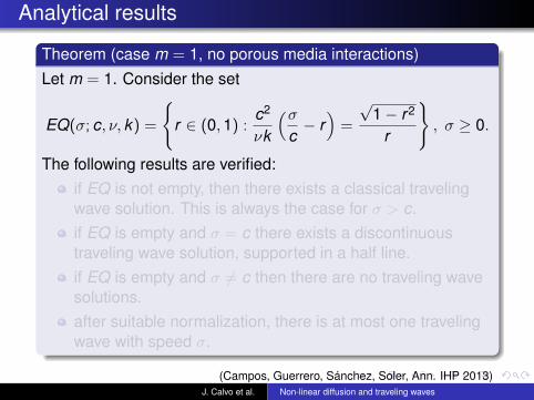
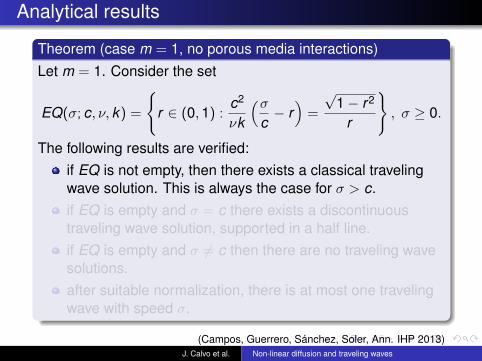
Theorem (case m = 1, no porous media interactions)Let m = 1. Consider the set
EQ(σ; c, ν, k) =
{r ∈ (0,1) :
c2
νk
(σc− r)=
√1− r2
r
}, σ ≥ 0.
The following results are verified:if EQ is not empty, then there exists a classical travelingwave solution. This is always the case for σ > c.if EQ is empty and σ = c there exists a discontinuoustraveling wave solution, supported in a half line.if EQ is empty and σ 6= c then there are no traveling wavesolutions.after suitable normalization, there is at most one travelingwave with speed σ.
(Campos, Guerrero, Sánchez, Soler, Ann. IHP 2013)J. Calvo et al. Non-linear diffusion and traveling waves
Analytical results
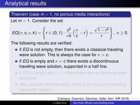
Theorem (case m = 1, no porous media interactions)Let m = 1. Consider the set
EQ(σ; c, ν, k) =
{r ∈ (0,1) :
c2
νk
(σc− r)=
√1− r2
r
}, σ ≥ 0.
The following results are verified:if EQ is not empty, then there exists a classical travelingwave solution. This is always the case for σ > c.if EQ is empty and σ = c there exists a discontinuoustraveling wave solution, supported in a half line.if EQ is empty and σ 6= c then there are no traveling wavesolutions.after suitable normalization, there is at most one travelingwave with speed σ.
(Campos, Guerrero, Sánchez, Soler, Ann. IHP 2013)J. Calvo et al. Non-linear diffusion and traveling waves

Analytical results
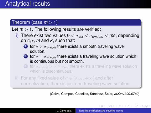
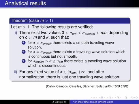
Theorem (case m > 1)Let m > 1. The following results are verified:
i) There exist two values 0 < σent < σsmooth < mc, dependingon c, ν,m and k , such that:
1 for σ > σsmooth there exists a smooth traveling wavesolution,
2 for σ = σsmooth there exists a traveling wave solution whichis continuous but not smooth,
3 for σsmooth > σ ≥ σent there exists a traveling wave solutionwhich is discontinuous.
ii) For any fixed value of σ ∈ [σent ,+∞[ and afternormalization, there is just one traveling wave solution.
(Calvo, Campos, Caselles, Sánchez, Soler, arXiv:1309.6789)
J. Calvo et al. Non-linear diffusion and traveling waves

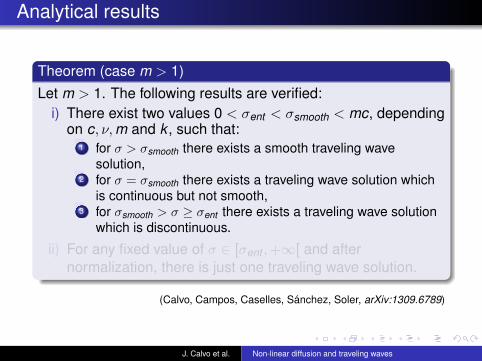
Analytical results
Theorem (case m > 1)Let m > 1. The following results are verified:
i) There exist two values 0 < σent < σsmooth < mc, dependingon c, ν,m and k , such that:
1 for σ > σsmooth there exists a smooth traveling wavesolution,
2 for σ = σsmooth there exists a traveling wave solution whichis continuous but not smooth,
3 for σsmooth > σ ≥ σent there exists a traveling wave solutionwhich is discontinuous.
ii) For any fixed value of σ ∈ [σent ,+∞[ and afternormalization, there is just one traveling wave solution.
(Calvo, Campos, Caselles, Sánchez, Soler, arXiv:1309.6789)
J. Calvo et al. Non-linear diffusion and traveling waves

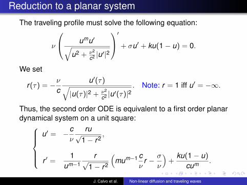
Reduction to a planar system
The traveling profile must solve the following equation:
ν
umu′√u2 + ν2
c2 |u′|2
′ + σu′ + ku(1− u) = 0.
We set
r(τ) = −νc
u′(τ)√|u(τ)|2 + ν2
c2 |u′(τ)|2. Note: r = 1 iff u′ = −∞.
Thus, the second order ODE is equivalent to a first order planardynamical system on a unit square:
u′ = −cν
ru√1− r2
,
r ′ =1
um−1r√
1− r2
(mum−1 c
νr − σ
ν
)+
ku(1− u)cum .
J. Calvo et al. Non-linear diffusion and traveling waves

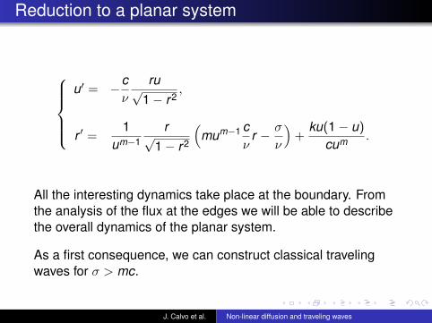
Reduction to a planar system
u′ = −c
ν
ru√1− r2
,
r ′ =1
um−1r√
1− r2
(mum−1 c
νr − σ
ν
)+
ku(1− u)cum .
All the interesting dynamics take place at the boundary. Fromthe analysis of the flux at the edges we will be able to describethe overall dynamics of the planar system.
As a first consequence, we can construct classical travelingwaves for σ > mc.
J. Calvo et al. Non-linear diffusion and traveling waves
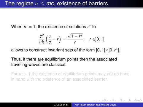
The regime σ ≤ mc, existence of barriers
When m = 1, the existence of solutions r∗ to
c2
νk
(σc− r)=
√1− r2
r, r ∈]0,1[
allows to construct invariant sets of the form ]0,1[×]0, r∗[.
Thus, if there are equilibrium points then the associatedtraveling waves are classical.
For m > 1 the existence of equilibrium points may not go handin hand with the existence of an associated barrier.
J. Calvo et al. Non-linear diffusion and traveling waves

The regime σ ≤ mc, breakdown of the classical theory
In this regime, orbits starting from the unstable manifold have achance to reach the upper edge of the planar domain.
Whenever this takes place, the profile develops an infinitetangent. Is it possible to get a reasonable solution out of this?
Recall that our profiles are monotonically decreasing. A wayout of the problem is to try to construct a profile with adownward jump discontinuity.
J. Calvo et al. Non-linear diffusion and traveling waves

The regime σ ≤ mc, breakdown of the classical theory
Distributional solutions to our model having a jump discontinuitymust satisfy the Rankine–Hugoniot jump condition:
V =F (u)+ − F (u)−
u+ − u−
V velocity at which the jump discontinuity movesu± values of the solution at both sides of the discontinuityF (u)± values of the flux at both sides of the discontinuity
J. Calvo et al. Non-linear diffusion and traveling waves
The regime σ ≤ mc, breakdown of the classical theory
Distributional solutions to our model having a jump discontinuitymust satisfy the Rankine–Hugoniot jump condition:
V =F (u)+ − F (u)−
u+ − u−
In our particular situation, this reduces to
σ = c(u+)m − (u−)m
u+ − u−
J. Calvo et al. Non-linear diffusion and traveling waves

The regime σ ≤ mc, breakdown of the classical theory
Distributional solutions to our model having a jump discontinuitymust satisfy the Rankine–Hugoniot jump condition:
V =F (u)+ − F (u)−
u+ − u−
In our particular situation, this reduces to
σ = c(u+)m − (u−)m
u+ − u−
Traveling waves that qualify as entropic solutions must satisfythis condition and must have infinite slopes at both sides of thediscontinuity.
This means that we can extend our singular profile using a neworbit starting from the set ]0,1[×{r = 1} or the zero state.
J. Calvo et al. Non-linear diffusion and traveling waves

About uniqueness
A uniqueness statement for solutions having the special form(t , x) 7→ u(x − σt) holds in the following class:
u is an entropy solution of the reaction-diffusion equation,u has its range in [0,1] and is not the state zero nor thestate one,there is a finite set of point pi such that u is smooth inR\{p1, . . . ,pn}.
Namely, given any value σ ≥ 0, there is at most one solution ofthe form (t , x) 7→ u(x − σt) in the former class (modulo spatialshifts). Note that no monotonicity assumptions on the profileare made: there are no traveling structures but the families oftraveling waves that we have constructed.
J. Calvo et al. Non-linear diffusion and traveling waves
Recap
A)u
ξ
1B)
u
ξ
1
C)u
ξ
1D)
u
ξ
1
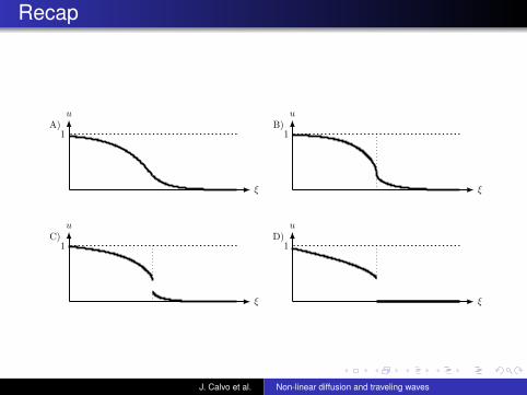
Figure 1: Travelling wave profiles for 2: A) σ > σsmooth, B) σ = σsmooth, C)σ ∈ (σent,σsmooth), D) σ = σent. Vertical dotted lines show singular tangentpoints. These profiles are in correspondence with the orbits depicted in Fig. 2B).
thus they encode processes in which the propagation of information (whateverit may be) takes place at finite speeds –see discussions elsewhere [].
The natural context where studying discontinuous solutions to flux–limitedporous media equations is the BV –theory as it has been analyzed in [7, 17, 18]which provides a suitable functional L1-framework that allows to treat suchsingular objects by means of the concept of entropy solutions.
2 Entropy solutions
Our purpose in this section is to state existence and uniqueness of entropy solu-tions of the reaction-diffusion equation (2). Moreover, we also give a geometricinterpretation of the entropy conditions on the jump set of the solutions. Equa-tion (2) belongs to the more general class of flux limited diffusion equations forwhich the correct concept of solution, permitting to prove existence and unique-ness results, is the notion of entropy solution [4, 17]. This class of equationswith F = 0 has been studied in a series of papers [3, 4, 6, 17, 18, 7] and for theso-called relativistic heat equation (m = 1 in (2)) with a Fisher–Kolmogorovtype reaction term in [5]. The notion of entropy solution is described in terms ofa set of inequalities of Kruzhkov’s type [31]. As proved in [18] when F = 0, theycan be characterized more geometrically on the jump set of the solution by say-ing that the graph of the function is vertical at those points. Our purpose is toextend these results to the case of (2) and a reaction term of Fisher–Kolmogorovtype. This will be fundamental to construct discontinuous traveling waves thatare entropy solutions of (2).
Our first purpose is to give a brief review of the concept of entropy solution
5
J. Calvo et al. Non-linear diffusion and traveling waves


![EN COORDENADAS ESFERICAS, DE LA ECUACION DE ONDAS ... · homogénea es el de ondas viajeras de D'Alembert [3]. Para el caso de ondas unidimensionales que se propagan en x existen](https://img.pdfslide.es/doc/110x75/5bbc609909d3f240128bc5d1/en-coordenadas-esfericas-de-la-ecuacion-de-ondas-homogenea-es-el-de-ondas.jpg)